Regresion lineal multiple
rlm.RdAjusta el modelo de regresion lineal multiple de acuerdo a la especificacion y ~ x1 + x2 + ...
Usage
rlm(
  f,
  data = NULL,
  pred = NULL,
  grf = TRUE,
  dfout = FALSE,
  alfa = 0.05,
  conf = 1 - alfa,
  decs = 3
)
Arguments
- f
formula: especificacion del modelo (ej. y ~ x1 + x2)
- data
data.frame: data table
- pred
data.frame: regressors for model prediction
- grf
logical: if grf=FALSE, graphical output is omitted
- dfout
logical: if dfout=TRUE, the procedure returns the data matrix with residuals and predictions
- alfa
real < 1: alpha error (parameter alternatively to confidence level). Default = 0.05.
- conf
real < 1: confidence level for effect estimation IC. Default = 1-alfa.
- decs
integer: decimal precision for results. Default = 3.
Value
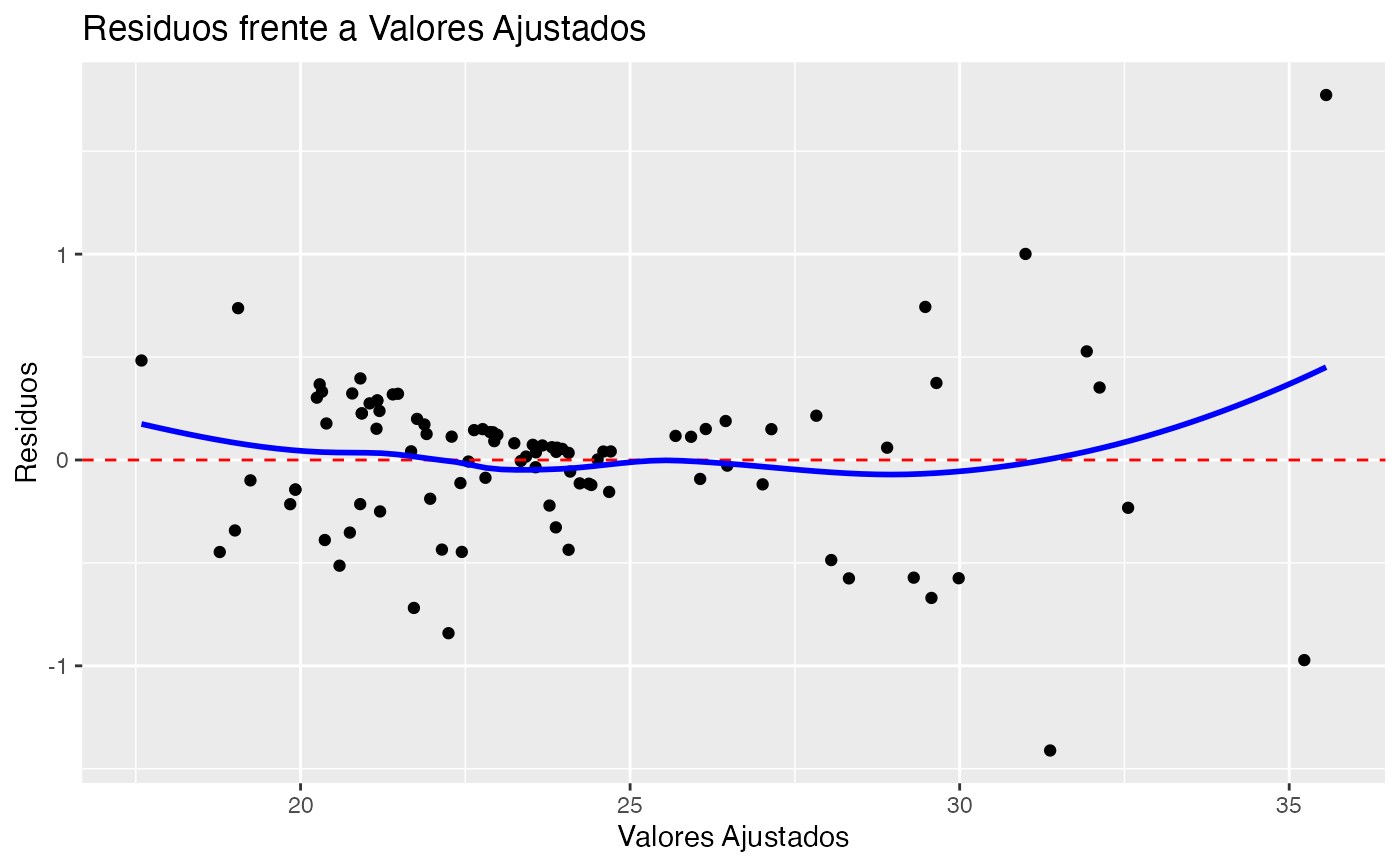
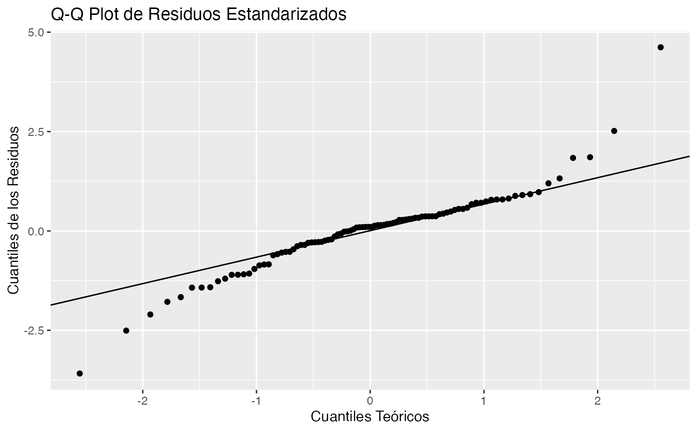
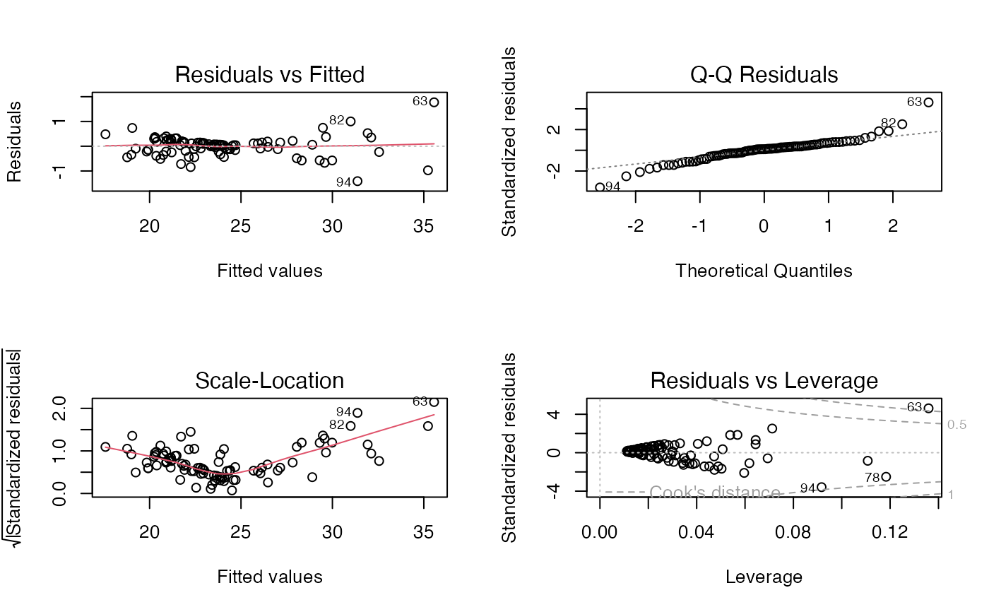
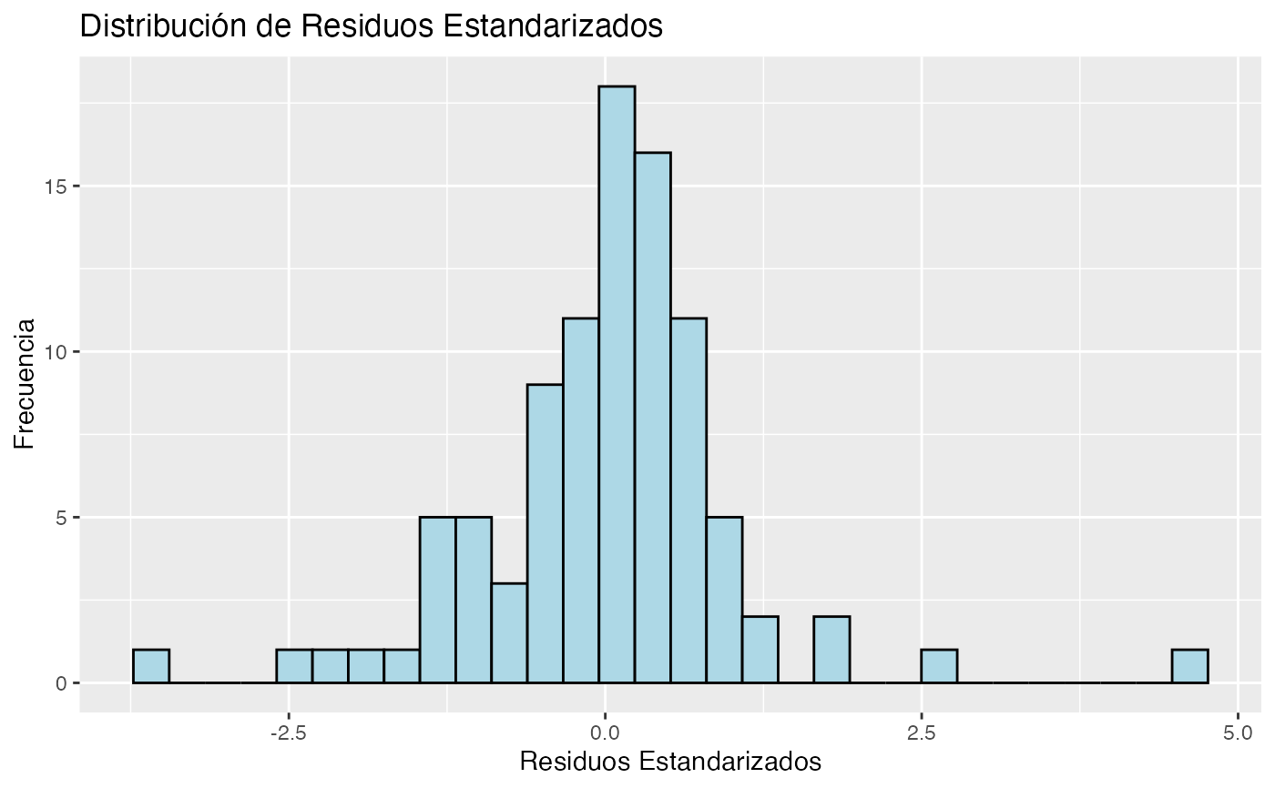
Report with descriptive measures, parameter estimation for multiple linear regression, residual description, and diagnostic plots
References
Montgomery, D. C., Peck, E. A., & Vining, G. G. (2012). Introduction to Linear Regression Analysis.
Examples
# Example 1 - Basic usage
data(osteo)
rlm(imc ~ peso + talla, data = osteo)
#>
#> Regresión lineal múltiple
#> ----------------------------------------------------------------
#> # Información muestral ---
#>
#> Variable n Media DT Min Max
#> imc imc 94 23.921 3.748 18.07 37.333
#> peso peso 94 63.839 11.804 44.60 99.000
#> talla talla 94 163.181 8.795 144.00 190.000
#>
#> # Modelo lineal ---
#>
#> Modelo : imc ~ peso + talla
#> R² = 0.988 (R² ajustado = 0.988 )
#> S²residual = 0.17
#>
#> Coeficientes del modelo :
#>
#> Termino Estimacion Error_Std IC_inf IC_sup t_exp sig
#> 1 (Intercept) 48.884 0.835 47.225 50.543 58.522 < 0.001
#> 2 peso 0.380 0.004 0.371 0.389 86.971 < 0.001
#> 3 talla -0.302 0.006 -0.313 -0.290 -51.431 < 0.001
#>
#> # Distribución residual ---
#> Error estándar residual: 0.413
#> Residuos Res_Est
#> min -1.411 -3.587
#> Q1 -0.180 -0.442
#> Q2 0.042 0.102
#> Q3 0.186 0.456
#> max 1.773 4.620
#>
#> Test de normalidad residual (Shapiro-Wilk):
#> w = 0.926 , < 0.001
#>


 # Example 2 - With predictions
data(osteo)
new_data <- data.frame(peso = c(70, 80), talla = c(170, 180))
rlm(imc ~ peso + talla, data = osteo, pred = new_data)
#>
#> Regresión lineal múltiple
#> ----------------------------------------------------------------
#> # Información muestral ---
#>
#> Variable n Media DT Min Max
#> imc imc 94 23.921 3.748 18.07 37.333
#> peso peso 94 63.839 11.804 44.60 99.000
#> talla talla 94 163.181 8.795 144.00 190.000
#>
#> # Modelo lineal ---
#>
#> Modelo : imc ~ peso + talla
#> R² = 0.988 (R² ajustado = 0.988 )
#> S²residual = 0.17
#>
#> Coeficientes del modelo :
#>
#> Termino Estimacion Error_Std IC_inf IC_sup t_exp sig
#> 1 (Intercept) 48.884 0.835 47.225 50.543 58.522 < 0.001
#> 2 peso 0.380 0.004 0.371 0.389 86.971 < 0.001
#> 3 talla -0.302 0.006 -0.313 -0.290 -51.431 < 0.001
#>
#> # Pronósticos con el modelo ---
#> Pronosticos puntuales y bandas al 95 % de confianza para
#> promedios IC(m), y para una nueva observación: IC(obs)
#>
#> peso talla Puntual IC_m_inf IC_m_sup IC_obs_inf IC_obs_sup
#> 1 70 170 24.20513 24.09751 24.31276 23.37811 25.03216
#> 2 80 180 24.98938 24.80351 25.17525 24.14859 25.83018
#>
#> # Distribución residual ---
#> Error estándar residual: 0.413
#> Residuos Res_Est
#> min -1.411 -3.587
#> Q1 -0.180 -0.442
#> Q2 0.042 0.102
#> Q3 0.186 0.456
#> max 1.773 4.620
#>
#> Test de normalidad residual (Shapiro-Wilk):
#> w = 0.926 , < 0.001
#>
# Example 2 - With predictions
data(osteo)
new_data <- data.frame(peso = c(70, 80), talla = c(170, 180))
rlm(imc ~ peso + talla, data = osteo, pred = new_data)
#>
#> Regresión lineal múltiple
#> ----------------------------------------------------------------
#> # Información muestral ---
#>
#> Variable n Media DT Min Max
#> imc imc 94 23.921 3.748 18.07 37.333
#> peso peso 94 63.839 11.804 44.60 99.000
#> talla talla 94 163.181 8.795 144.00 190.000
#>
#> # Modelo lineal ---
#>
#> Modelo : imc ~ peso + talla
#> R² = 0.988 (R² ajustado = 0.988 )
#> S²residual = 0.17
#>
#> Coeficientes del modelo :
#>
#> Termino Estimacion Error_Std IC_inf IC_sup t_exp sig
#> 1 (Intercept) 48.884 0.835 47.225 50.543 58.522 < 0.001
#> 2 peso 0.380 0.004 0.371 0.389 86.971 < 0.001
#> 3 talla -0.302 0.006 -0.313 -0.290 -51.431 < 0.001
#>
#> # Pronósticos con el modelo ---
#> Pronosticos puntuales y bandas al 95 % de confianza para
#> promedios IC(m), y para una nueva observación: IC(obs)
#>
#> peso talla Puntual IC_m_inf IC_m_sup IC_obs_inf IC_obs_sup
#> 1 70 170 24.20513 24.09751 24.31276 23.37811 25.03216
#> 2 80 180 24.98938 24.80351 25.17525 24.14859 25.83018
#>
#> # Distribución residual ---
#> Error estándar residual: 0.413
#> Residuos Res_Est
#> min -1.411 -3.587
#> Q1 -0.180 -0.442
#> Q2 0.042 0.102
#> Q3 0.186 0.456
#> max 1.773 4.620
#>
#> Test de normalidad residual (Shapiro-Wilk):
#> w = 0.926 , < 0.001
#>

 # Example 3 - English output
data(osteo)
options(BioEstatR.lang = "en")
rlm(imc ~ peso + talla, data = osteo)
#>
#> Multiple Linear Regression
#> ----------------------------------------------------------------
#> # Sample information ---
#>
#> Variable n Media DT Min Max
#> imc imc 94 23.921 3.748 18.07 37.333
#> peso peso 94 63.839 11.804 44.60 99.000
#> talla talla 94 163.181 8.795 144.00 190.000
#>
#> # Linear model ---
#>
#> Model : imc ~ peso + talla
#> R² = 0.988 (R² adjusted = 0.988 )
#> S²residual = 0.17
#>
#> Model coefficients :
#>
#> Termino Estimacion Error_Std IC_inf IC_sup t_exp sig
#> 1 (Intercept) 48.884 0.835 47.225 50.543 58.522 < 0.001
#> 2 peso 0.380 0.004 0.371 0.389 86.971 < 0.001
#> 3 talla -0.302 0.006 -0.313 -0.290 -51.431 < 0.001
#>
#> # Distribución residual ---
#> Error estándar residual: 0.413
#> Residuos Res_Est
#> min -1.411 -3.587
#> Q1 -0.180 -0.442
#> Q2 0.042 0.102
#> Q3 0.186 0.456
#> max 1.773 4.620
#>
#> Test de normalidad residual (Shapiro-Wilk):
#> w = 0.926 , < 0.001
#>
# Example 3 - English output
data(osteo)
options(BioEstatR.lang = "en")
rlm(imc ~ peso + talla, data = osteo)
#>
#> Multiple Linear Regression
#> ----------------------------------------------------------------
#> # Sample information ---
#>
#> Variable n Media DT Min Max
#> imc imc 94 23.921 3.748 18.07 37.333
#> peso peso 94 63.839 11.804 44.60 99.000
#> talla talla 94 163.181 8.795 144.00 190.000
#>
#> # Linear model ---
#>
#> Model : imc ~ peso + talla
#> R² = 0.988 (R² adjusted = 0.988 )
#> S²residual = 0.17
#>
#> Model coefficients :
#>
#> Termino Estimacion Error_Std IC_inf IC_sup t_exp sig
#> 1 (Intercept) 48.884 0.835 47.225 50.543 58.522 < 0.001
#> 2 peso 0.380 0.004 0.371 0.389 86.971 < 0.001
#> 3 talla -0.302 0.006 -0.313 -0.290 -51.431 < 0.001
#>
#> # Distribución residual ---
#> Error estándar residual: 0.413
#> Residuos Res_Est
#> min -1.411 -3.587
#> Q1 -0.180 -0.442
#> Q2 0.042 0.102
#> Q3 0.186 0.456
#> max 1.773 4.620
#>
#> Test de normalidad residual (Shapiro-Wilk):
#> w = 0.926 , < 0.001
#>


 options(BioEstatR.lang = "es")