Copyright (c) 2017
THE SOFTWARE IS PROVIDED "AS IS", WITHOUT WARRANTY OF ANY KIND, EXPRESS OR
IMPLIED, INCLUDING BUT NOT LIMITED TO THE WARRANTIES OF MERCHANTABILITY,
FITNESS FOR A PARTICULAR PURPOSE AND NON INFRINGEMENT. IN NO EVENT SHALL THE
AUTHORS OR COPYRIGHT HOLDERS BE LIABLE FOR ANY CLAIM, DAMAGES OR OTHER
LIABILITY, WHETHER IN AN ACTION OF CONTRACT, TORT OR OTHERWISE, ARISING FROM,
OUT OF OR IN CONNECTION WITH THE SOFTWARE OR THE USE OR OTHER DEALINGS IN
THE SOFTWARE.
Bug reports: miguel.luque.easp at juntadeandalucia.es
. set more off

. use https://stats.idre.ucla.edu/stat/examples/asa2/whas100, clear

. label define status 0 "alive" 1 "dead"

. label value folstatus status

. label define gender 0 "male" 1 "female"

. label value gender gender

. label var addate "Admission date"

. label var foldate "Follow up date"

. label var hosstay "Length of Hospital Stay in days"

. label var foltime "Follow Up Time"

. label var folstatus "Vital Status"

. describe

Contains data from https://stats.idre.ucla.edu/stat/examples/asa2/whas100.dta
  obs:           100
 vars:             9                          5 Nov 2007 15:59
 size:         2,700
----------------------------------------------------------------------------------------------
              storage   display    value
variable name   type    format     label      variable label
----------------------------------------------------------------------------------------------
id              byte    %8.0g
addate          str8    %9s                   Admission date
foldate         str8    %9s                   Follow up date
hosstay         byte    %8.0g                 Length of Hospital Stay in days
foltime         int     %8.0g                 Follow Up Time
folstatus       byte    %8.0g      status     Vital Status
age             byte    %8.0g
gender          byte    %8.0g      gender
bmi             float   %9.0g
----------------------------------------------------------------------------------------------
Sorted by:

. list, sep(0) noobs

  +------------------------------------------------------------------------------------+
  |  id     addate    foldate   hosstay   foltime   folsta~s   age   gender        bmi |
  |------------------------------------------------------------------------------------|
  |   1    3/13/95    3/19/95         4         6       dead    65     male   31.38134 |
  |   2    1/14/95    1/23/96         5       374       dead    88   female    22.6579 |
  |   3    2/17/95    10/4/01         5      2421       dead    77     male   27.87892 |
  |   4     4/7/95    7/14/95         9        98       dead    81   female   21.47878 |
  |   5     2/9/95    5/29/98         4      1205       dead    78     male   30.70601 |
  |   6    1/16/95    9/11/00         7      2065       dead    82   female   26.45294 |
  |   7    1/17/95   10/15/97         3      1002       dead    66   female   35.71147 |
  |   8   11/15/94   11/24/00        56      2201       dead    81   female   28.27676 |
  |   9    8/18/95    2/23/96         5       189       dead    76     male   27.12082 |
  |  10    7/22/95   12/31/02         9      2719      alive    40     male   21.78971 |
  |  11   10/11/95   12/31/02         6      2638      alive    73   female   28.43344 |
  |  12    5/26/95    9/29/96        11       492       dead    83     male   24.66175 |
  |  13    5/21/95    3/18/96         6       302       dead    64   female   27.46412 |
  |  14   12/14/95   12/31/02        10      2574      alive    58     male   29.83756 |
  |  15    11/8/95   12/31/02         7      2610      alive    43     male   22.95776 |
  |  16    10/8/95   12/31/02         5      2641      alive    39     male   30.10881 |
  |  17   10/17/95    5/12/00         6      1669       dead    66     male   31.99738 |
  |  18   10/30/95     1/5/03         9      2624       dead    61     male    30.7142 |
  |  19   12/10/95   12/31/02         6      2578      alive    49     male   25.69548 |
  |  20   11/23/95   12/31/02         5      2595      alive    53   female   30.12017 |
  |  21    10/5/95     2/5/96         6       123       dead    85     male   18.41038 |
  |  22    11/5/95   12/31/02         8      2613      alive    69   female   37.60097 |
  |  23     9/9/95   10/22/97         4       774       dead    54     male   28.97529 |
  |  24     9/9/95    3/13/01        14      2012       dead    82     male   19.90095 |
  |  25   12/15/95   12/31/02         4      2573      alive    67   female   28.32237 |
  |  26    12/3/95    1/19/01        11      1874       dead    89   female   23.43605 |
  |  27   10/18/95   12/31/02         2      2631      alive    68     male   26.44693 |
  |  28    3/16/95     6/4/00         7      1907       dead    78     male   28.20595 |
  |  29   10/25/95    4/15/97         5       538       dead    56     male   24.11997 |
  |  30    10/6/95    1/18/96         4       104       dead    85   female   36.71647 |
  |  31     9/3/95     9/9/95         4         6       dead    72     male   27.97907 |
  |  32    6/30/95     5/1/99         5      1401       dead    50     male     20.363 |
  |  33    7/22/95   12/22/02         8      2710       dead    81   female   28.64898 |
  |  34    9/17/95     1/5/98         4       841       dead    85   female   20.17772 |
  |  35    3/21/97    8/16/97         6       148       dead    84   female    23.6187 |
  |  36    2/23/97   12/31/02        12      2137      alive    75     male   23.67519 |
  |  37     1/1/97   12/31/02        16      2190      alive    61     male    23.4314 |
  |  38    1/18/97   12/31/02         5      2173      alive    48     male    33.4511 |
  |  39    1/19/97    4/25/98         8       461       dead    83   female   19.57068 |
  |  40    3/18/97   12/31/02        10      2114      alive    82     male   25.82748 |
  |  41     2/3/97   12/31/02         4      2157      alive    62     male   30.86625 |
  |  42    5/17/97   12/31/02         5      2054      alive    39     male   24.21079 |
  |  43     3/8/97   12/31/02         5      2124      alive    45     male   31.66439 |
  |  44    2/23/97   12/31/02         4      2137      alive    65     male   26.22085 |
  |  45    6/14/97     1/5/03        18      2031       dead    76   female   32.41986 |
  |  46     7/7/97   12/31/02         9      2003      alive    77   female   24.56345 |
  |  47    4/27/97   12/31/02         9      2074      alive    68     male    21.3055 |
  |  48    5/15/97    2/13/98         7       274       dead    73     male   26.45678 |
  |  49    7/26/97   12/31/02         4      1984      alive    64     male   27.97977 |
  |  50    7/17/97   12/31/02         6      1993      alive    80     male   36.02333 |
  |  51     9/9/97   12/31/02         7      1939      alive    84   female   22.31424 |
  |  52    6/19/97     9/3/00         4      1172       dead    43   female   25.33148 |
  |  53    8/20/97   11/17/97         3        89       dead    87   female   18.77718 |
  |  54    8/28/97     1/3/98         7       128       dead    70   female   18.60004 |
  |  55     9/9/97   12/31/02        17      1939      alive    80     male   25.50204 |
  |  56     9/1/97    9/15/97        11        14       dead    64   female   24.41255 |
  |  57     9/3/97    6/10/00         5      1011       dead    59   female   29.85998 |
  |  58    9/24/97   10/30/01         6      1497       dead    92     male    24.3664 |
  |  59    9/19/97   12/31/02         3      1929      alive    51     male   34.77034 |
  |  60    4/17/97   12/31/02         1      2084      alive    41     male   27.26234 |
  |  61   10/21/97     2/5/98         6       107       dead    90     male   24.78423 |
  |  62    10/2/97   12/27/98         4       451       dead    83     male   21.80987 |
  |  63     1/8/97   12/31/02         3      2183      alive    61     male   27.36909 |
  |  64   11/11/97   12/31/02         7      1876      alive    64     male   26.22085 |
  |  65    11/7/97    5/31/00         3       936       dead    82     male   26.88683 |
  |  66    4/20/97    4/18/98         5       363       dead    91   female   27.61844 |
  |  67    6/18/97     5/1/00         5      1048       dead    48     male   31.58373 |
  |  68   10/29/97   12/31/02        12      1889      alive    63     male   23.33267 |
  |  69    4/29/97   12/31/02         5      2072      alive    81     male   28.35006 |
  |  70    11/8/97   12/31/02         7      1879      alive    52     male   32.63621 |
  |  71   11/17/97   12/31/02         4      1870      alive    65     male   31.95113 |
  |  72   11/28/97   12/31/02         5      1859      alive    74     male   25.01782 |
  |  73    5/19/97   12/31/02         5      2052      alive    62     male   30.22827 |
  |  74   12/11/97   12/31/02         4      1846      alive    60   female   29.28812 |
  |  75    5/10/97   12/31/02         7      2061      alive    71     male   32.32407 |
  |  76    10/6/97   12/31/02         3      1912      alive    73     male   31.47445 |
  |  77   12/21/97   12/31/02         5      1836      alive    43     male   28.59188 |
  |  78   11/22/97    3/16/98         7       114       dead    80     male   33.36074 |
  |  79   10/31/97     2/4/02         7      1557       dead    72     male   21.80987 |
  |  80    6/28/97   12/27/00         5      1278       dead    57     male   23.57087 |
  |  81   12/21/97   12/31/02         3      1836      alive    80   female   28.35006 |
  |  82    10/2/97   12/31/02         6      1916      alive    76     male   28.03555 |
  |  83    9/14/97   12/31/02         3      1934      alive    53     male   24.21079 |
  |  84    9/25/97   12/31/02        10      1923      alive    44     male   32.60387 |
  |  85    12/2/97    1/15/98         3        44       dead    71     male    23.0563 |
  |  86    9/26/97   12/31/02         6      1922      alive    64     male   31.75016 |
  |  87   10/24/97    7/25/98         5       274       dead    86     male   21.10959 |
  |  88   11/27/97   12/31/02         7      1860      alive    72   female   25.23266 |
  |  89    4/12/97    3/23/02         4      1806       dead    73   female   22.86698 |
  |  90    2/15/97   12/31/02         6      2145      alive    85   female   26.05501 |
  |  91   10/22/97    4/22/98         5       182       dead    60     male   23.18023 |
  |  92    6/27/97   12/31/02         4      2013      alive    63     male   35.48949 |
  |  93    1/17/97   12/31/02         5      2174      alive    80   female   20.59809 |
  |  94   12/12/97    5/24/02         4      1624       dead    74     male   30.13206 |
  |  95    11/4/97    5/10/98        10       187       dead    79   female   16.78615 |
  |  96    11/4/97   12/31/02         4      1883      alive    48   female   32.11709 |
  |  97   12/24/97    4/19/02         3      1577       dead    32   female   39.93835 |
  |  98   11/26/97    1/27/98         8        62       dead    86   female   14.91878 |
  |  99    8/10/97   12/31/02        16      1969      alive    56     male   29.05295 |
  | 100    3/26/97    2/13/00         7      1054       dead    74     male   32.89087 |
  +------------------------------------------------------------------------------------+
. gen entry = date(addate, "MD19Y")

. format entry %td

. gen exit = date(foldate, "MDY", 2003)

. format exit %td

. stset exit, fail(folstatus==1) enter(time entry) origin(time entry) // Scale in days

     failure event:  folstatus == 1
obs. time interval:  (origin, exit]
 enter on or after:  time entry
 exit on or before:  failure
    t for analysis:  (time-origin)
            origin:  time entry

------------------------------------------------------------------------------
        100  total observations
          0  exclusions
------------------------------------------------------------------------------
        100  observations remaining, representing
         51  failures in single-record/single-failure data
    150,540  total analysis time at risk and under observation
                                                at risk from t =         0
                                     earliest observed entry t =         0
                                          last observed exit t =     2,719

. stdescribe // In days

         failure _d:  folstatus == 1
   analysis time _t:  (exit-origin)
             origin:  time entry
  enter on or after:  time entry

                                   |-------------- per subject --------------|
Category                   total        mean         min     median        max
------------------------------------------------------------------------------
no. of subjects              100
no. of records               100           1           1          1          1

(first) entry time                         0           0          0          0
(final) exit time                     1505.4           6     1877.5       2719

subjects with gap              0
time on gap if gap             0
time at risk              150540      1505.4           6     1877.5       2719

failures                      51         .51           0          1          1
------------------------------------------------------------------------------

. stset exit, fail(folstatus==1) enter(time entry) origin(time entry) scale(365.25) // Scale i
> n years

     failure event:  folstatus == 1
obs. time interval:  (origin, exit]
 enter on or after:  time entry
 exit on or before:  failure
    t for analysis:  (time-origin)/365.25
            origin:  time entry

------------------------------------------------------------------------------
        100  total observations
          0  exclusions
------------------------------------------------------------------------------
        100  observations remaining, representing
         51  failures in single-record/single-failure data
    412.156  total analysis time at risk and under observation
                                                at risk from t =         0
                                     earliest observed entry t =         0
                                          last observed exit t =  7.444216

. stdescribe // In years

         failure _d:  folstatus == 1
   analysis time _t:  (exit-origin)/365.25
             origin:  time entry
  enter on or after:  time entry

                                   |-------------- per subject --------------|
Category                   total        mean         min     median        max
------------------------------------------------------------------------------
no. of subjects              100
no. of records               100           1           1          1          1

(first) entry time                         0           0          0          0
(final) exit time                   4.121561    .0164271   5.140315   7.444216

subjects with gap              0
time on gap if gap             0
time at risk           412.15606    4.121561    .0164271   5.140315   7.444216

failures                      51         .51           0          1          1
------------------------------------------------------------------------------

. stset foltime, fail(folstatus==1) scale(365.25) // Using the computed time

     failure event:  folstatus == 1
obs. time interval:  (0, foltime]
 exit on or before:  failure
    t for analysis:  time/365.25

------------------------------------------------------------------------------
        100  total observations
          0  exclusions
------------------------------------------------------------------------------
        100  observations remaining, representing
         51  failures in single-record/single-failure data
    412.156  total analysis time at risk and under observation
                                                at risk from t =         0
                                     earliest observed entry t =         0
                                          last observed exit t =  7.444216

. stdescribe // In years

         failure _d:  folstatus == 1
   analysis time _t:  foltime/365.25

                                   |-------------- per subject --------------|
Category                   total        mean         min     median        max
------------------------------------------------------------------------------
no. of subjects              100
no. of records               100           1           1          1          1

(first) entry time                         0           0          0          0
(final) exit time                   4.121561    .0164271   5.140315   7.444216

subjects with gap              0
time on gap if gap             0
time at risk           412.15606    4.121561    .0164271   5.140315   7.444216

failures                      51         .51           0          1          1
------------------------------------------------------------------------------

. stvary // For multiple records

         failure _d:  folstatus == 1
   analysis time _t:  foltime/365.25

               subjects for whom the variable is
                                                 never    always   sometimes
    variable |  constant    varying             missing   missing   missing
-------------+--------------------------------------------------------------
          id |       100          0                 100         0         0
      addate |       100          0                 100         0         0
     foldate |       100          0                 100         0         0
     hosstay |       100          0                 100         0         0
         age |       100          0                 100         0         0
      gender |       100          0                 100         0         0
         bmi |       100          0                 100         0         0
       entry |       100          0                 100         0         0
        exit |       100          0                 100         0         0
. sum foltime

    Variable |        Obs        Mean    Std. Dev.       Min        Max
-------------+---------------------------------------------------------
     foltime |        100      1505.4    858.8992          6       2719

. gen yrfol = foltime/365.25

. sum yrfol

    Variable |        Obs        Mean    Std. Dev.       Min        Max
-------------+---------------------------------------------------------
       yrfol |        100    4.121561    2.351538   .0164271   7.444216

. egen catyrfol = cut(yrfol), at(0,2,4,6,8)

. tab catyrfol

   catyrfol |      Freq.     Percent        Cum.
------------+-----------------------------------
          0 |         25       25.00       25.00
          2 |         11       11.00       36.00
          4 |         50       50.00       86.00
          6 |         14       14.00      100.00
------------+-----------------------------------
      Total |        100      100.00

. stset catyrfol, fail(folstatus==1)

     failure event:  folstatus == 1
obs. time interval:  (0, catyrfol]
 exit on or before:  failure

------------------------------------------------------------------------------
        100  total observations
         25  observations end on or before enter()
------------------------------------------------------------------------------
         75  observations remaining, representing
         26  failures in single-record/single-failure data
        306  total analysis time at risk and under observation
                                                at risk from t =         0
                                     earliest observed entry t =         0
                                          last observed exit t =         6

. sts list //Kaplan-Meier

         failure _d:  folstatus == 1
   analysis time _t:  catyrfol

           Beg.          Net            Survivor      Std.
  Time    Total   Fail   Lost           Function     Error     [95% Conf. Int.]
-------------------------------------------------------------------------------
     2       75     11      0             0.8533    0.0409     0.7508    0.9160
     4       64     11     39             0.7067    0.0526     0.5895    0.7960
     6       14      4     10             0.5048    0.0932     0.3132    0.6686
-------------------------------------------------------------------------------

. sts list, cumhaz //Cumulative Hazard

         failure _d:  folstatus == 1
   analysis time _t:  catyrfol

           Beg.          Net          Nelson-Aalen    Std.
  Time    Total   Fail   Lost           Cum. Haz.    Error     [95% Conf. Int.]
-------------------------------------------------------------------------------
     2       75     11      0             0.1467    0.0442     0.0812    0.2648
     4       64     11     39             0.3185    0.0681     0.2095    0.4844
     6       14      4     10             0.6043    0.1583     0.3616    1.0097
-------------------------------------------------------------------------------
\[ \hat{S}(t)\,=\,\prod_{(j|t_{j}\leq t)} \left(\frac{n_{j}\,-\,d_{j}}{n_{j}}\right) \]
. qui: stset foltime, fail(folstatus==1) scale(365.25) // Using the computed time

.
. sts graph

         failure _d:  folstatus == 1
   analysis time _t:  foltime/365.25
. sts generate svar = s

.
. sts graph, risktable

         failure _d:  folstatus == 1
   analysis time _t:  foltime/365.25

. sts graph, by(gender) risktable

         failure _d:  folstatus == 1
   analysis time _t:  foltime/365.25

. stci

         failure _d:  folstatus == 1
   analysis time _t:  foltime/365.25

             |    no. of
             |  subjects         50%     Std. Err.     [95% Conf. Interval]
-------------+-------------------------------------------------------------
       total |       100     6.02601      .5603603      4.44627    7.41958

. stci, p(25)

         failure _d:  folstatus == 1
   analysis time _t:  foltime/365.25

             |    no. of
             |  subjects         25%     Std. Err.     [95% Conf. Interval]
-------------+-------------------------------------------------------------
       total |       100    1.472964      .7682197      .750171    3.29911
. stsum //Overall Incidence Rate and PTR (use it for your abstract and the results section of
> your paper)

         failure _d:  folstatus == 1
   analysis time _t:  foltime/365.25

         |               incidence       no. of    |------ Survival time -----|
         | time at risk     rate        subjects        25%       50%       75%
---------+---------------------------------------------------------------------
   total |  412.1560575   .1237395           100   1.472964   6.02601  7.419576

. stsum, by(gender) //By levels of your categorical variables. Note 95%CI is not provided
>

         failure _d:  folstatus == 1
   analysis time _t:  foltime/365.25

         |               incidence       no. of    |------ Survival time -----|
gender   | time at risk     rate        subjects        25%       50%       75%
---------+---------------------------------------------------------------------
    male |  284.2299795   .0985118            65   2.885695   7.18412         .
  female |   127.926078   .1797913            35   .8268309  4.944559  7.419576
---------+---------------------------------------------------------------------
   total |  412.1560575   .1237395           100   1.472964   6.02601  7.419576
\[ H(t)\,=\,\sum_{(j|t_{j}\leq t)}\frac{d_{j}}{n_{j}} \]
. sts graph, cumhaz

         failure _d:  folstatus == 1
   analysis time _t:  foltime/365.25

. sts graph, cumhaz by(gender)

         failure _d:  folstatus == 1
   analysis time _t:  foltime/365.25

. sum yrfol // Y = Mean followup x N = Years at risk

    Variable |        Obs        Mean    Std. Dev.       Min        Max
-------------+---------------------------------------------------------
       yrfol |        100    4.121561    2.351538   .0164271   7.444216

. strate //    Y = 412.2 years at risk and Incidence Density or Rate per person-year at risk

         failure _d:  folstatus == 1
   analysis time _t:  foltime/365.25

Estimated rates and lower/upper bounds of 95% confidence intervals
(100 records included in the analysis)

  +------------------------------------------------+
  |  D          Y       Rate      Lower      Upper |
  |------------------------------------------------|
  | 51   412.1561   0.123740   0.094041   0.162817 |
  +------------------------------------------------+


.
. gen n = 1

. tabrate folstatus gender, exp(n) per(1000) // Cumulative incidence (Proportion) over 8 years

table of cases (D), person-years (Y), and rates per 1000 person-years

  +--------------------------------------------------+
  | gender   _D     _Y     _rate    ci_low   ci_high |
  |--------------------------------------------------|
  |   male   28   65.0   430.769   297.429   623.888 |
  | female   23   35.0   657.143   436.689   988.889 |
  +--------------------------------------------------+

Chisq test for unequal rates =     2.29 (1 df, p =  0.131 )

.
. strate gender, per(1000) // Incidence Density or Rate per 1000 person-year at risk

         failure _d:  folstatus == 1
   analysis time _t:  foltime/365.25

Estimated rates (per 1000) and lower/upper bounds of 95% confidence intervals
(100 records included in the analysis)

  +----------------------------------------------------+
  | gender    D        Y      Rate     Lower     Upper |
  |----------------------------------------------------|
  |   male   28   0.2842    98.512    68.018   142.676 |
  | female   23   0.1279   179.791   119.476   270.556 |
  +----------------------------------------------------+


. stmh gender, c(1,0)

         failure _d:  folstatus == 1
   analysis time _t:  foltime/365.25

Maximum likelihood estimate of the rate ratio
  comparing gender==1 vs. gender==0

RR estimate, and lower and upper 95% confidence limits

        ----------------------------------------------------------
             RR       chi2        P>chi2      [95% Conf. Interval]
        ----------------------------------------------------------
          1.825       4.71        0.0300         1.051      3.168
        ----------------------------------------------------------
. stmh gender, by(age) c(1,0)

         failure _d:  folstatus == 1
   analysis time _t:  foltime/365.25

Maximum likelihood estimate of the rate ratio
  comparing gender==1 vs. gender==0
  by age

RR estimate, and lower and upper 95% confidence limits

  +----------------------------+
  | age     RR   Lower   Upper |
  |----------------------------|
  |  43      .       .       . |
  |  48   0.00       .       . |
  |  60   0.00       .       . |
  |  64      .       .       . |
  |  66   1.67    0.10   26.63 |
  |----------------------------|
  |  72   0.00       .       . |
  |  73   0.49    0.03    7.86 |
  |  76   1.04    0.06   16.57 |
  |  77   0.00       .       . |
  |  80   0.00       .       . |
  |----------------------------|
  |  81      .       .       . |
  |  82   1.23    0.11   13.52 |
  |  83   1.02    0.09   11.28 |
  |  85   0.08    0.01    0.88 |
  |  86   4.42    0.28   70.65 |
  +----------------------------+

Overall estimate controlling for age

        ----------------------------------------------------------
             RR       chi2        P>chi2      [95% Conf. Interval]
        ----------------------------------------------------------
          1.009       0.00        0.9765         0.543      1.877
        ----------------------------------------------------------

Approx test for unequal RRs (effect modification): chi2(14) =    65.21
                                                   Pr>chi2 =   0.0000
\[ H(t)\,=\,-\text{ln}\left[\text(S(t))\right] \]
\[ S(t)\,=\,\text{exp}\left[\text(-H(t))\right] \]
. sts generate kmS = s // Obtain KM survivor estimate

. sts generate naH = na // Obtain NA cum. hazard estimate

. gen naS = exp(-naH) // Calculate NA survivor estimate

. gen kmH = -log(kmS) // Calculate KM cum. harzard estimate

. label var kmS "KM"

. label var naS "exp(-NA)"

. label var kmH "-log(KM)"

. label var naH "NA"

. twoway connected kmS naS _t, connect(J J) sort // Survivor estimate using NA always > than K
> M (simulations)
")
. twoway connected kmH naH _t, connect(J J) sort

. sts list, by(gender) compare // Survival

         failure _d:  folstatus == 1
   analysis time _t:  foltime/365.25

                 Survivor Function
gender             male     female
----------------------------------
time       0     1.0000     1.0000
     .928474     0.8462     0.7429
     1.85695     0.8000     0.6571
     2.78542     0.7692     0.5714
     3.71389     0.7077     0.5429
     4.64237     0.6308     0.5143
     5.57084     0.5872     0.4059
     6.49932     0.5872     0.3007
     7.42779     0.3854          .
     8.35626          .          .
----------------------------------

. sts list, na by(gender) compare // Cumulative Hazard

         failure _d:  folstatus == 1
   analysis time _t:  foltime/365.25

            Nelson-Aalen Cum. Haz.
gender             male     female
----------------------------------
time       0     0.0000     0.0000
     .928474     0.1651     0.2924
     1.85695     0.2207     0.4125
     2.78542     0.2595     0.5490
     3.71389     0.3420     0.5990
     4.64237     0.4558     0.6517
     5.57084     0.5260     0.8787
     6.49932     0.5260     1.1564
     7.42779     0.9010          .
     8.35626          .          .
----------------------------------

. sts test gender, logrank // Logrank Test (it is an extension of the Mantel-Haenszel applied
> to survival)

         failure _d:  folstatus == 1
   analysis time _t:  foltime/365.25


Log-rank test for equality of survivor functions

       |   Events         Events
gender |  observed       expected
-------+-------------------------
male   |        28          34.62
female |        23          16.38
-------+-------------------------
Total  |        51          51.00

             chi2(1) =       3.97
             Pr>chi2 =     0.0463
. sum age

    Variable |        Obs        Mean    Std. Dev.       Min        Max
-------------+---------------------------------------------------------
         age |        100       68.25    14.42807         32         92

. egen agecat = cut(age), at(30,50,80,100)

. sts graph, by(agecat) risktable gwood

         failure _d:  folstatus == 1
   analysis time _t:  foltime/365.25

. sts test agecat, trend logrank

         failure _d:  folstatus == 1
   analysis time _t:  foltime/365.25


Log-rank test for equality of survivor functions

       |   Events         Events
agecat |  observed       expected
-------+-------------------------
30     |         3           9.75
50     |        26          28.91
80     |        22          12.34
-------+-------------------------
Total  |        51          51.00

             chi2(2) =      12.73
             Pr>chi2 =     0.0017

Test for trend of survivor functions

             chi2(1) =      12.73
             Pr>chi2 =     0.0004
. sts list // very small number of ties failure _d: folstatus == 1 analysis time _t: foltime/365.25 Beg. Net Survivor Std. Time Total Fail Lost Function Error [95% Conf. Int.] ------------------------------------------------------------------------------- .0164 100 2 0 0.9800 0.0140 0.9224 0.9950 .0383 98 1 0 0.9700 0.0171 0.9099 0.9902 .1205 97 1 0 0.9600 0.0196 0.8969 0.9848 .1697 96 1 0 0.9500 0.0218 0.8840 0.9789 .2437 95 1 0 0.9400 0.0237 0.8713 0.9726 .2683 94 1 0 0.9300 0.0255 0.8588 0.9660 .2847 93 1 0 0.9200 0.0271 0.8464 0.9592 .293 92 1 0 0.9100 0.0286 0.8342 0.9521 .3121 91 1 0 0.9000 0.0300 0.8221 0.9449 .3368 90 1 0 0.8900 0.0313 0.8102 0.9375 .3504 89 1 0 0.8800 0.0325 0.7984 0.9300 .4052 88 1 0 0.8700 0.0336 0.7867 0.9224 .4983 87 1 0 0.8600 0.0347 0.7751 0.9146 .512 86 1 0 0.8500 0.0357 0.7636 0.9067 .5175 85 1 0 0.8400 0.0367 0.7522 0.8988 .7502 84 2 0 0.8200 0.0384 0.7296 0.8826 .8268 82 1 0 0.8100 0.0392 0.7185 0.8743 .9938 81 1 0 0.8000 0.0400 0.7074 0.8660 1.024 80 1 0 0.7900 0.0407 0.6964 0.8577 1.235 79 1 0 0.7800 0.0414 0.6854 0.8492 1.262 78 1 0 0.7700 0.0421 0.6745 0.8407 1.347 77 1 0 0.7600 0.0427 0.6637 0.8322 1.473 76 1 0 0.7500 0.0433 0.6529 0.8236 2.119 75 1 0 0.7400 0.0439 0.6422 0.8149 2.303 74 1 0 0.7300 0.0444 0.6315 0.8061 2.563 73 1 0 0.7200 0.0449 0.6209 0.7974 2.743 72 1 0 0.7100 0.0454 0.6103 0.7885 2.768 71 1 0 0.7000 0.0458 0.5998 0.7797 2.869 70 1 0 0.6900 0.0462 0.5894 0.7707 2.886 69 1 0 0.6800 0.0466 0.5790 0.7617 3.209 68 1 0 0.6700 0.0470 0.5686 0.7527 3.299 67 1 0 0.6600 0.0474 0.5583 0.7437 3.499 66 1 0 0.6500 0.0477 0.5480 0.7345 3.836 65 1 0 0.6400 0.0480 0.5377 0.7254 4.099 64 1 0 0.6300 0.0483 0.5275 0.7162 4.263 63 1 0 0.6200 0.0485 0.5174 0.7070 4.318 62 1 0 0.6100 0.0488 0.5073 0.6977 4.446 61 1 0 0.6000 0.0490 0.4972 0.6884 4.569 60 1 0 0.5900 0.0492 0.4872 0.6790 4.945 59 1 0 0.5800 0.0494 0.4772 0.6696 5.027 58 0 2 0.5800 0.0494 0.4772 0.6696 5.054 56 0 1 0.5800 0.0494 0.4772 0.6696 5.09 55 0 1 0.5800 0.0494 0.4772 0.6696 5.092 54 0 1 0.5800 0.0494 0.4772 0.6696 5.12 53 0 1 0.5800 0.0494 0.4772 0.6696 5.131 52 1 0 0.5688 0.0497 0.4658 0.6593 5.136 51 0 1 0.5688 0.0497 0.4658 0.6593 5.144 50 0 1 0.5688 0.0497 0.4658 0.6593 5.155 49 0 1 0.5688 0.0497 0.4658 0.6593 5.172 48 0 1 0.5688 0.0497 0.4658 0.6593 5.221 47 1 0 0.5567 0.0500 0.4533 0.6482 5.235 46 0 1 0.5567 0.0500 0.4533 0.6482 5.246 45 0 1 0.5567 0.0500 0.4533 0.6482 5.262 44 0 1 0.5567 0.0500 0.4533 0.6482 5.265 43 0 1 0.5567 0.0500 0.4533 0.6482 5.281 42 0 1 0.5567 0.0500 0.4533 0.6482 5.295 41 0 1 0.5567 0.0500 0.4533 0.6482 5.309 40 0 2 0.5567 0.0500 0.4533 0.6482 5.391 38 0 1 0.5567 0.0500 0.4533 0.6482 5.432 37 0 1 0.5567 0.0500 0.4533 0.6482 5.457 36 0 1 0.5567 0.0500 0.4533 0.6482 5.484 35 0 1 0.5567 0.0500 0.4533 0.6482 5.509 34 1 0 0.5404 0.0512 0.4351 0.6343 5.511 33 0 1 0.5404 0.0512 0.4351 0.6343 5.561 32 1 0 0.5235 0.0523 0.4165 0.6198 5.618 31 0 1 0.5235 0.0523 0.4165 0.6198 5.624 30 0 1 0.5235 0.0523 0.4165 0.6198 5.643 29 0 1 0.5235 0.0523 0.4165 0.6198 5.654 28 1 0 0.5048 0.0537 0.3956 0.6041 5.673 27 0 1 0.5048 0.0537 0.3956 0.6041 5.678 26 0 1 0.5048 0.0537 0.3956 0.6041 5.706 25 0 1 0.5048 0.0537 0.3956 0.6041 5.788 24 0 1 0.5048 0.0537 0.3956 0.6041 5.815 23 0 1 0.5048 0.0537 0.3956 0.6041 5.851 22 0 2 0.5048 0.0537 0.3956 0.6041 5.873 20 0 1 0.5048 0.0537 0.3956 0.6041 5.906 19 0 1 0.5048 0.0537 0.3956 0.6041 5.949 18 0 1 0.5048 0.0537 0.3956 0.6041 5.952 17 0 1 0.5048 0.0537 0.3956 0.6041 5.977 16 0 1 0.5048 0.0537 0.3956 0.6041 5.996 15 0 1 0.5048 0.0537 0.3956 0.6041 6.026 14 1 0 0.4687 0.0607 0.3466 0.5816 6.628 13 1 0 0.4327 0.0659 0.3023 0.5562 7.044 12 0 1 0.4327 0.0659 0.3023 0.5562 7.047 11 0 1 0.4327 0.0659 0.3023 0.5562 7.058 10 0 1 0.4327 0.0659 0.3023 0.5562 7.105 9 0 1 0.4327 0.0659 0.3023 0.5562 7.146 8 0 1 0.4327 0.0659 0.3023 0.5562 7.154 7 0 1 0.4327 0.0659 0.3023 0.5562 7.184 6 1 0 0.3606 0.0857 0.1997 0.5241 7.203 5 0 1 0.3606 0.0857 0.1997 0.5241 7.222 4 0 1 0.3606 0.0857 0.1997 0.5241 7.231 3 0 1 0.3606 0.0857 0.1997 0.5241 7.42 2 1 0 0.1803 0.1345 0.0179 0.4820 7.444 1 0 1 0.1803 0.1345 0.0179 0.4820 ------------------------------------------------------------------------------- . stcox gender // Breslow estimate for ties failure _d: folstatus == 1 analysis time _t: foltime/365.25 Iteration 0: log likelihood = -209.11972 Iteration 1: log likelihood = -207.2544 Iteration 2: log likelihood = -207.2423 Iteration 3: log likelihood = -207.2423 Refining estimates: Iteration 0: log likelihood = -207.2423 Cox regression -- Breslow method for ties No. of subjects = 100 Number of obs = 100 No. of failures = 51 Time at risk = 412.1560575 LR chi2(1) = 3.75 Log likelihood = -207.2423 Prob > chi2 = 0.0527 ------------------------------------------------------------------------------ _t | Haz. Ratio Std. Err. z P>|z| [95% Conf. Interval] -------------+---------------------------------------------------------------- gender | 1.742761 .4921308 1.97 0.049 1.002006 3.031133 ------------------------------------------------------------------------------ . stcox gender, efron // Mor accurate than Breslow failure _d: folstatus == 1 analysis time _t: foltime/365.25 Iteration 0: log likelihood = -209.09769 Iteration 1: log likelihood = -207.23669 Iteration 2: log likelihood = -207.22467 Iteration 3: log likelihood = -207.22467 Refining estimates: Iteration 0: log likelihood = -207.22467 Cox regression -- Efron method for ties No. of subjects = 100 Number of obs = 100 No. of failures = 51 Time at risk = 412.1560575 LR chi2(1) = 3.75 Log likelihood = -207.22467 Prob > chi2 = 0.0529 ------------------------------------------------------------------------------ _t | Haz. Ratio Std. Err. z P>|z| [95% Conf. Interval] -------------+---------------------------------------------------------------- gender | 1.741613 .4918126 1.96 0.049 1.00134 3.029157 ------------------------------------------------------------------------------ . . . stcox i.gender // Indicator variables failure _d: folstatus == 1 analysis time _t: foltime/365.25 Iteration 0: log likelihood = -209.11972 Iteration 1: log likelihood = -207.2544 Iteration 2: log likelihood = -207.2423 Iteration 3: log likelihood = -207.2423 Refining estimates: Iteration 0: log likelihood = -207.2423 Cox regression -- Breslow method for ties No. of subjects = 100 Number of obs = 100 No. of failures = 51 Time at risk = 412.1560575 LR chi2(1) = 3.75 Log likelihood = -207.2423 Prob > chi2 = 0.0527 ------------------------------------------------------------------------------ _t | Haz. Ratio Std. Err. z P>|z| [95% Conf. Interval] -------------+---------------------------------------------------------------- gender | female | 1.742761 .4921308 1.97 0.049 1.002006 3.031133 ------------------------------------------------------------------------------ . . tab agecat agecat | Freq. Percent Cum. ------------+----------------------------------- 30 | 14 14.00 14.00 50 | 56 56.00 70.00 80 | 30 30.00 100.00 ------------+----------------------------------- Total | 100 100.00 . stcox i.agecat // Categorical variables (Contrast indicator and wald test) failure _d: folstatus == 1 analysis time _t: foltime/365.25 Iteration 0: log likelihood = -209.11972 Iteration 1: log likelihood = -203.05446 Iteration 2: log likelihood = -202.59595 Iteration 3: log likelihood = -202.59206 Iteration 4: log likelihood = -202.59206 Refining estimates: Iteration 0: log likelihood = -202.59206 Cox regression -- Breslow method for ties No. of subjects = 100 Number of obs = 100 No. of failures = 51 Time at risk = 412.1560575 LR chi2(2) = 13.06 Log likelihood = -202.59206 Prob > chi2 = 0.0015 ------------------------------------------------------------------------------ _t | Haz. Ratio Std. Err. z P>|z| [95% Conf. Interval] -------------+---------------------------------------------------------------- agecat | 50 | 2.950289 1.807422 1.77 0.077 .8879672 9.802395 80 | 5.934847 3.668544 2.88 0.004 1.767059 19.93279 ------------------------------------------------------------------------------ . . stcox age // Continuous variables interpretation and scale failure _d: folstatus == 1 analysis time _t: foltime/365.25 Iteration 0: log likelihood = -209.11972 Iteration 1: log likelihood = -200.64424 Iteration 2: log likelihood = -200.44425 Iteration 3: log likelihood = -200.44391 Refining estimates: Iteration 0: log likelihood = -200.44391 Cox regression -- Breslow method for ties No. of subjects = 100 Number of obs = 100 No. of failures = 51 Time at risk = 412.1560575 LR chi2(1) = 17.35 Log likelihood = -200.44391 Prob > chi2 = 0.0000 ------------------------------------------------------------------------------ _t | Haz. Ratio Std. Err. z P>|z| [95% Conf. Interval] -------------+---------------------------------------------------------------- age | 1.04672 .0125089 3.82 0.000 1.022488 1.071527 ------------------------------------------------------------------------------ . gen age5 = age/5 . stcox age5 failure _d: folstatus == 1 analysis time _t: foltime/365.25 Iteration 0: log likelihood = -209.11972 Iteration 1: log likelihood = -200.64424 Iteration 2: log likelihood = -200.44425 Iteration 3: log likelihood = -200.44391 Refining estimates: Iteration 0: log likelihood = -200.44391 Cox regression -- Breslow method for ties No. of subjects = 100 Number of obs = 100 No. of failures = 51 Time at risk = 412.1560575 LR chi2(1) = 17.35 Log likelihood = -200.44391 Prob > chi2 = 0.0000 ------------------------------------------------------------------------------ _t | Haz. Ratio Std. Err. z P>|z| [95% Conf. Interval] -------------+---------------------------------------------------------------- age5 | 1.256473 .0750778 3.82 0.000 1.117613 1.412586 ------------------------------------------------------------------------------ . . stcox c.age##c.age // Functional form age: No evidence of nonlinear effect (quadratic) failure _d: folstatus == 1 analysis time _t: foltime/365.25 Iteration 0: log likelihood = -209.11972 Iteration 1: log likelihood = -200.17407 Iteration 2: log likelihood = -199.58078 Iteration 3: log likelihood = -199.57967 Iteration 4: log likelihood = -199.57967 Refining estimates: Iteration 0: log likelihood = -199.57967 Cox regression -- Breslow method for ties No. of subjects = 100 Number of obs = 100 No. of failures = 51 Time at risk = 412.1560575 LR chi2(2) = 19.08 Log likelihood = -199.57967 Prob > chi2 = 0.0001 ------------------------------------------------------------------------------ _t | Haz. Ratio Std. Err. z P>|z| [95% Conf. Interval] -------------+---------------------------------------------------------------- age | .9222841 .0850547 -0.88 0.380 .7697777 1.105005 | c.age#c.age | 1.000944 .000689 1.37 0.170 .9995945 1.002295 ------------------------------------------------------------------------------ . . stcox i.gender##c.age // Interactions: small evidence effect modification of age failure _d: folstatus == 1 analysis time _t: foltime/365.25 Iteration 0: log likelihood = -209.11972 Iteration 1: log likelihood = -199.57097 Iteration 2: log likelihood = -198.9633 Iteration 3: log likelihood = -198.95656 Iteration 4: log likelihood = -198.95655 Refining estimates: Iteration 0: log likelihood = -198.95655 Cox regression -- Breslow method for ties No. of subjects = 100 Number of obs = 100 No. of failures = 51 Time at risk = 412.1560575 LR chi2(3) = 20.33 Log likelihood = -198.95655 Prob > chi2 = 0.0001 ------------------------------------------------------------------------------ _t | Haz. Ratio Std. Err. z P>|z| [95% Conf. Interval] -------------+---------------------------------------------------------------- gender | female | 25.7504 47.048 1.78 0.075 .717088 924.6889 age | 1.06086 .0171645 3.65 0.000 1.027746 1.095041 | gender#c.age | female | .959227 .0234825 -1.70 0.089 .9142888 1.006374 ------------------------------------------------------------------------------ . . stcox i.gender age // Age as confounder. Note: consider the interpretation of gender failure _d: folstatus == 1 analysis time _t: foltime/365.25 Iteration 0: log likelihood = -209.11972 Iteration 1: log likelihood = -200.5215 Iteration 2: log likelihood = -200.3233 Iteration 3: log likelihood = -200.323 Refining estimates: Iteration 0: log likelihood = -200.323 Cox regression -- Breslow method for ties No. of subjects = 100 Number of obs = 100 No. of failures = 51 Time at risk = 412.1560575 LR chi2(2) = 17.59 Log likelihood = -200.323 Prob > chi2 = 0.0002 ------------------------------------------------------------------------------ _t | Haz. Ratio Std. Err. z P>|z| [95% Conf. Interval] -------------+---------------------------------------------------------------- gender | female | 1.16075 .351101 0.49 0.622 .6416069 2.099946 age | 1.044538 .0132085 3.45 0.001 1.018968 1.07075 ------------------------------------------------------------------------------ . . gen age30 = age - 30 . stcox i.gender age30 // More meaninful interpretation (mean centering age) failure _d: folstatus == 1 analysis time _t: foltime/365.25 Iteration 0: log likelihood = -209.11972 Iteration 1: log likelihood = -200.5215 Iteration 2: log likelihood = -200.3233 Iteration 3: log likelihood = -200.323 Refining estimates: Iteration 0: log likelihood = -200.323 Cox regression -- Breslow method for ties No. of subjects = 100 Number of obs = 100 No. of failures = 51 Time at risk = 412.1560575 LR chi2(2) = 17.59 Log likelihood = -200.323 Prob > chi2 = 0.0002 ------------------------------------------------------------------------------ _t | Haz. Ratio Std. Err. z P>|z| [95% Conf. Interval] -------------+---------------------------------------------------------------- gender | female | 1.16075 .351101 0.49 0.622 .6416069 2.099946 age30 | 1.044538 .0132085 3.45 0.001 1.018968 1.07075 ------------------------------------------------------------------------------ . . stcox gender // Likelihood Ratio Test failure _d: folstatus == 1 analysis time _t: foltime/365.25 Iteration 0: log likelihood = -209.11972 Iteration 1: log likelihood = -207.2544 Iteration 2: log likelihood = -207.2423 Iteration 3: log likelihood = -207.2423 Refining estimates: Iteration 0: log likelihood = -207.2423 Cox regression -- Breslow method for ties No. of subjects = 100 Number of obs = 100 No. of failures = 51 Time at risk = 412.1560575 LR chi2(1) = 3.75 Log likelihood = -207.2423 Prob > chi2 = 0.0527 ------------------------------------------------------------------------------ _t | Haz. Ratio Std. Err. z P>|z| [95% Conf. Interval] -------------+---------------------------------------------------------------- gender | 1.742761 .4921308 1.97 0.049 1.002006 3.031133 ------------------------------------------------------------------------------ . estimates store A . stcox gender age failure _d: folstatus == 1 analysis time _t: foltime/365.25 Iteration 0: log likelihood = -209.11972 Iteration 1: log likelihood = -200.5215 Iteration 2: log likelihood = -200.3233 Iteration 3: log likelihood = -200.323 Refining estimates: Iteration 0: log likelihood = -200.323 Cox regression -- Breslow method for ties No. of subjects = 100 Number of obs = 100 No. of failures = 51 Time at risk = 412.1560575 LR chi2(2) = 17.59 Log likelihood = -200.323 Prob > chi2 = 0.0002 ------------------------------------------------------------------------------ _t | Haz. Ratio Std. Err. z P>|z| [95% Conf. Interval] -------------+---------------------------------------------------------------- gender | 1.16075 .351101 0.49 0.622 .6416069 2.099946 age | 1.044538 .0132085 3.45 0.001 1.018968 1.07075 ------------------------------------------------------------------------------ . estimates store B . lrtest A B Likelihood-ratio test LR chi2(1) = 13.84 (Assumption: A nested in B) Prob > chi2 = 0.0002 . . tab agecat gender, row chi // Do not forget crosstabulations: understanding your data is KEY > ! +----------------+ | Key | |----------------| | frequency | | row percentage | +----------------+ | gender agecat | male female | Total -----------+----------------------+---------- 30 | 11 3 | 14 | 78.57 21.43 | 100.00 -----------+----------------------+---------- 50 | 41 15 | 56 | 73.21 26.79 | 100.00 -----------+----------------------+---------- 80 | 13 17 | 30 | 43.33 56.67 | 100.00 -----------+----------------------+---------- Total | 65 35 | 100 | 65.00 35.00 | 100.00 Pearson chi2(2) = 8.9848 Pr = 0.011
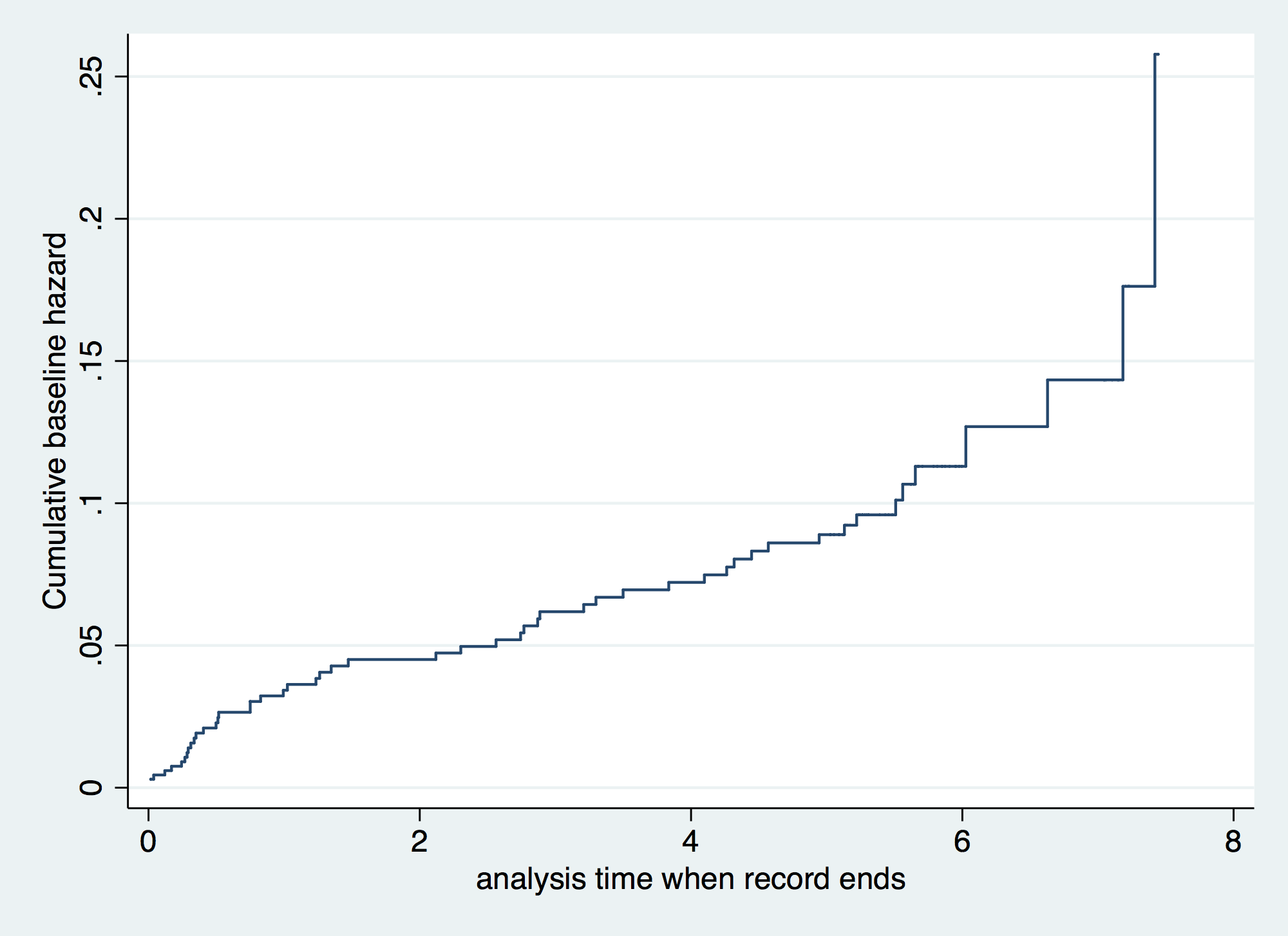
. stcox gender age30

         failure _d:  folstatus == 1
   analysis time _t:  foltime/365.25

Iteration 0:   log likelihood = -209.11972
Iteration 1:   log likelihood =  -200.5215
Iteration 2:   log likelihood =  -200.3233
Iteration 3:   log likelihood =   -200.323
Refining estimates:
Iteration 0:   log likelihood =   -200.323

Cox regression -- Breslow method for ties

No. of subjects =          100                  Number of obs    =         100
No. of failures =           51
Time at risk    =  412.1560575
                                                LR chi2(2)       =       17.59
Log likelihood  =     -200.323                  Prob > chi2      =      0.0002

------------------------------------------------------------------------------
          _t | Haz. Ratio   Std. Err.      z    P>|z|     [95% Conf. Interval]
-------------+----------------------------------------------------------------
      gender |    1.16075    .351101     0.49   0.622     .6416069    2.099946
       age30 |   1.044538   .0132085     3.45   0.001     1.018968     1.07075
------------------------------------------------------------------------------

.
. predict H0, basechazard // Baseline cumulative hazard function

. tw line H0 _t, connect (J) sort
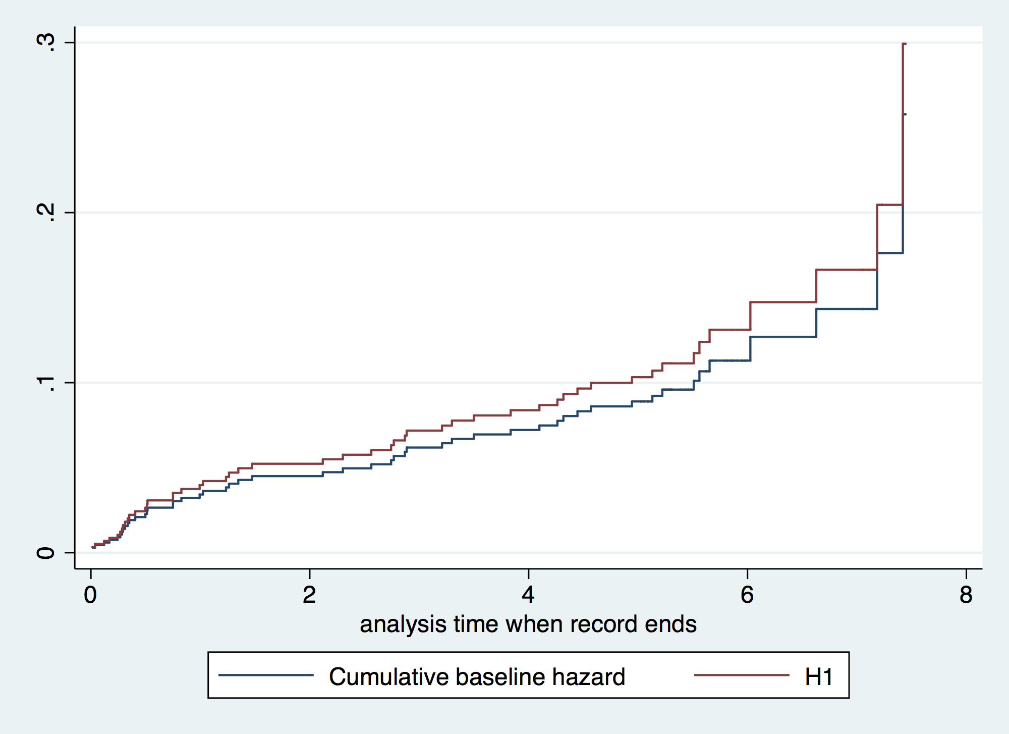
. gen H1 = H0*exp(_b[gender]) // Baseline cumulative hazard by gender

. tw line H0 H1 _t, connect (J J) sort
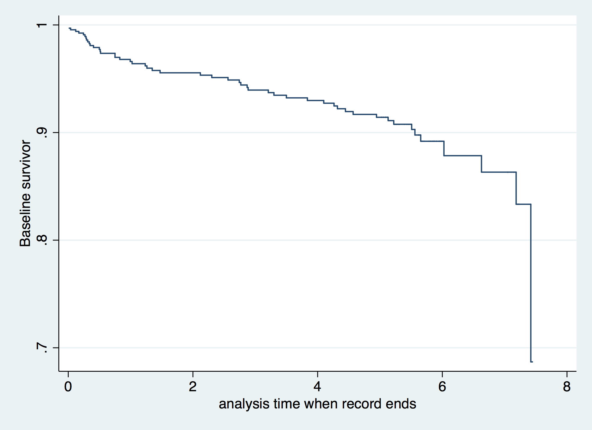
. predict S0, basesurv // Baseline Survivor function

. tw line S _t, connect (J) sort
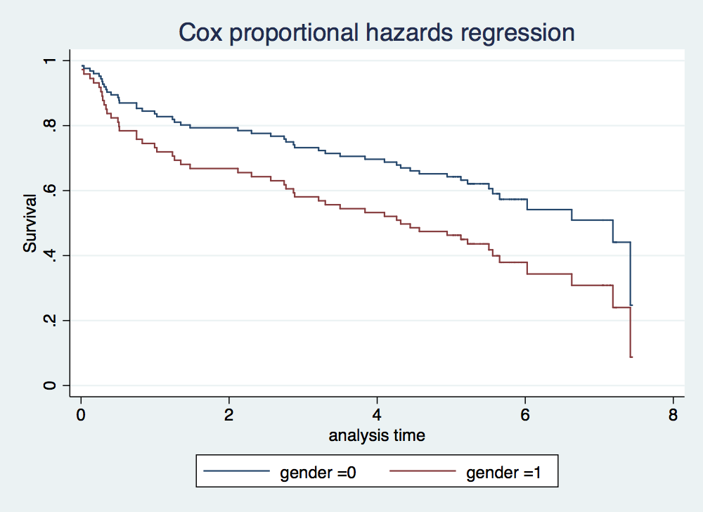
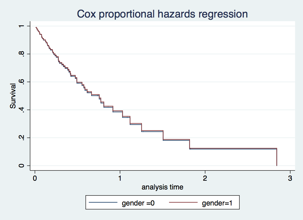
. stcox gender

         failure _d:  folstatus == 1
   analysis time _t:  foltime/365.25

Iteration 0:   log likelihood = -209.11972
Iteration 1:   log likelihood =  -207.2544
Iteration 2:   log likelihood =  -207.2423
Iteration 3:   log likelihood =  -207.2423
Refining estimates:
Iteration 0:   log likelihood =  -207.2423

Cox regression -- Breslow method for ties

No. of subjects =          100                  Number of obs    =         100
No. of failures =           51
Time at risk    =  412.1560575
                                                LR chi2(1)       =        3.75
Log likelihood  =    -207.2423                  Prob > chi2      =      0.0527

------------------------------------------------------------------------------
          _t | Haz. Ratio   Std. Err.      z    P>|z|     [95% Conf. Interval]
-------------+----------------------------------------------------------------
      gender |   1.742761   .4921308     1.97   0.049     1.002006    3.031133
------------------------------------------------------------------------------

. stcurve, surv at1(gender =0) at2(gender =1)
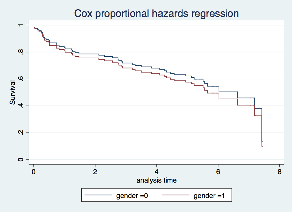
. stcox gender age

         failure _d:  folstatus == 1
   analysis time _t:  foltime/365.25

Iteration 0:   log likelihood = -209.11972
Iteration 1:   log likelihood =  -200.5215
Iteration 2:   log likelihood =  -200.3233
Iteration 3:   log likelihood =   -200.323
Refining estimates:
Iteration 0:   log likelihood =   -200.323

Cox regression -- Breslow method for ties

No. of subjects =          100                  Number of obs    =         100
No. of failures =           51
Time at risk    =  412.1560575
                                                LR chi2(2)       =       17.59
Log likelihood  =     -200.323                  Prob > chi2      =      0.0002

------------------------------------------------------------------------------
          _t | Haz. Ratio   Std. Err.      z    P>|z|     [95% Conf. Interval]
-------------+----------------------------------------------------------------
      gender |    1.16075    .351101     0.49   0.622     .6416069    2.099946
         age |   1.044538   .0132085     3.45   0.001     1.018968     1.07075
------------------------------------------------------------------------------

. stcurve, surv at1(gender =0) at2(gender =1)
. estat phtest // There is no evidence that the model violates the proportional-hazards assump
> tion

      Test of proportional-hazards assumption

      Time:  Time
      ----------------------------------------------------------------
                  |                      chi2       df       Prob>chi2
      ------------+---------------------------------------------------
      global test |                      0.36        2         0.8353
      ----------------------------------------------------------------

. estat phtest, detail

      Test of proportional-hazards assumption

      Time:  Time
      ----------------------------------------------------------------
                  |       rho            chi2       df       Prob>chi2
      ------------+---------------------------------------------------
      gender      |     -0.06680         0.27        1         0.6010
      age         |     -0.01167         0.01        1         0.9204
      ------------+---------------------------------------------------
      global test |                      0.36        2         0.8353
      ----------------------------------------------------------------
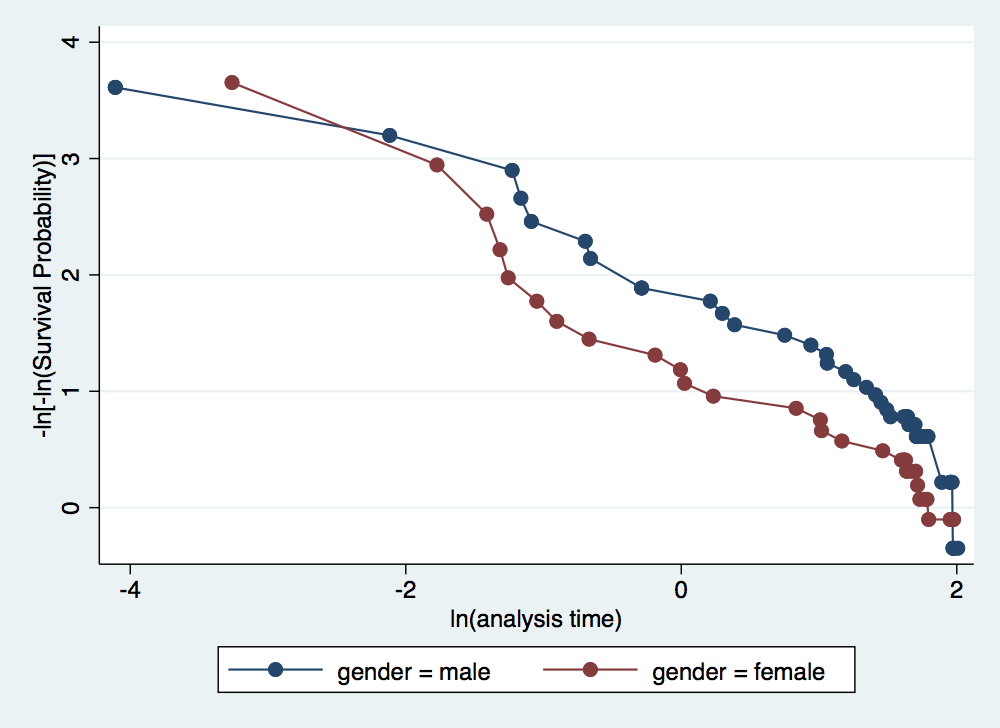
. stphplot, by(gender) adjust(age) //Curves are roughly parallel, providing evidence in favor
> of the proportional hazard assumption of gender

         failure _d:  folstatus == 1
   analysis time _t:  foltime/365.25
. stcox gender age

         failure _d:  folstatus == 1
   analysis time _t:  foltime/365.25

Iteration 0:   log likelihood = -209.11972
Iteration 1:   log likelihood =  -200.5215
Iteration 2:   log likelihood =  -200.3233
Iteration 3:   log likelihood =   -200.323
Refining estimates:
Iteration 0:   log likelihood =   -200.323

Cox regression -- Breslow method for ties

No. of subjects =          100                  Number of obs    =         100
No. of failures =           51
Time at risk    =  412.1560575
                                                LR chi2(2)       =       17.59
Log likelihood  =     -200.323                  Prob > chi2      =      0.0002

------------------------------------------------------------------------------
          _t | Haz. Ratio   Std. Err.      z    P>|z|     [95% Conf. Interval]
-------------+----------------------------------------------------------------
      gender |    1.16075    .351101     0.49   0.622     .6416069    2.099946
         age |   1.044538   .0132085     3.45   0.001     1.018968     1.07075
------------------------------------------------------------------------------

. stcox age, strata(gender)

         failure _d:  folstatus == 1
   analysis time _t:  foltime/365.25

Iteration 0:   log likelihood = -173.10245
Iteration 1:   log likelihood = -166.56589
Iteration 2:   log likelihood = -166.39683
Iteration 3:   log likelihood =  -166.3966
Refining estimates:
Iteration 0:   log likelihood =  -166.3966

Stratified Cox regr. -- Breslow method for ties

No. of subjects =          100                  Number of obs    =         100
No. of failures =           51
Time at risk    =  412.1560575
                                                LR chi2(1)       =       13.41
Log likelihood  =    -166.3966                  Prob > chi2      =      0.0003

------------------------------------------------------------------------------
          _t | Haz. Ratio   Std. Err.      z    P>|z|     [95% Conf. Interval]
-------------+----------------------------------------------------------------
         age |   1.044398   .0133473     3.40   0.001     1.018563    1.070889
------------------------------------------------------------------------------
                                                          Stratified by gender
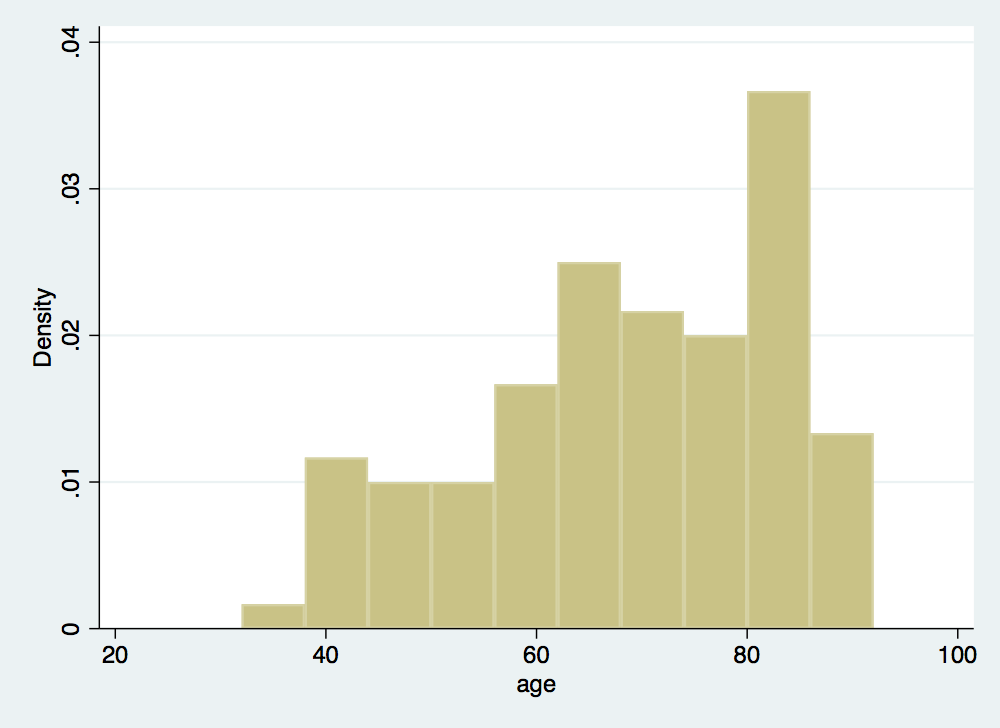
. hist age
(bin=10, start=32, width=6)
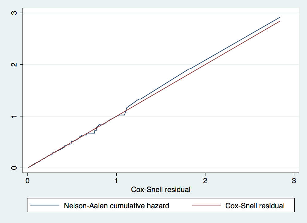
. stcox gender age

         failure _d:  folstatus == 1
   analysis time _t:  foltime/365.25

Iteration 0:   log likelihood = -209.11972
Iteration 1:   log likelihood =  -200.5215
Iteration 2:   log likelihood =  -200.3233
Iteration 3:   log likelihood =   -200.323
Refining estimates:
Iteration 0:   log likelihood =   -200.323

Cox regression -- Breslow method for ties

No. of subjects =          100                  Number of obs    =         100
No. of failures =           51
Time at risk    =  412.1560575
                                                LR chi2(2)       =       17.59
Log likelihood  =     -200.323                  Prob > chi2      =      0.0002

------------------------------------------------------------------------------
          _t | Haz. Ratio   Std. Err.      z    P>|z|     [95% Conf. Interval]
-------------+----------------------------------------------------------------
      gender |    1.16075    .351101     0.49   0.622     .6416069    2.099946
         age |   1.044538   .0132085     3.45   0.001     1.018968     1.07075
------------------------------------------------------------------------------

. predict cs, csnell //Cox-Snell residuals have a standard censored exponential distribution w
> ith hazard ratio of one

. stset cs, fail(folstatus)

     failure event:  folstatus != 0 & folstatus < .
obs. time interval:  (0, cs]
 exit on or before:  failure

------------------------------------------------------------------------------
        100  total observations
          0  exclusions
------------------------------------------------------------------------------
        100  observations remaining, representing
         51  failures in single-record/single-failure data
         51  total analysis time at risk and under observation
                                                at risk from t =         0
                                     earliest observed entry t =         0
                                          last observed exit t =  2.761897

. sts gen Hcs = na

. tw line Hcs cs cs, sort

. gen lnage = ln(age)

. drop Hcs cs

. stcox gender lnage

         failure _d:  folstatus
   analysis time _t:  cs

Iteration 0:   log likelihood =  -191.6887
Iteration 1:   log likelihood = -191.65715
Iteration 2:   log likelihood = -191.65714
Refining estimates:
Iteration 0:   log likelihood = -191.65714

Cox regression -- no ties

No. of subjects =          100                  Number of obs    =         100
No. of failures =           51
Time at risk    =  51.00000005
                                                LR chi2(2)       =        0.06
Log likelihood  =   -191.65714                  Prob > chi2      =      0.9689

------------------------------------------------------------------------------
          _t | Haz. Ratio   Std. Err.      z    P>|z|     [95% Conf. Interval]
-------------+----------------------------------------------------------------
      gender |   .9563769   .3030901    -0.14   0.888     .5138905    1.779867
       lnage |   .8683343    .730407    -0.17   0.867     .1669903    4.515258
------------------------------------------------------------------------------

. predict cs, csnell //Cox-Snell residuals

. stset cs, fail(folstatus)

     failure event:  folstatus != 0 & folstatus < .
obs. time interval:  (0, cs]
 exit on or before:  failure

------------------------------------------------------------------------------
        100  total observations
          0  exclusions
------------------------------------------------------------------------------
        100  observations remaining, representing
         51  failures in single-record/single-failure data
         51  total analysis time at risk and under observation
                                                at risk from t =         0
                                     earliest observed entry t =         0
                                          last observed exit t =  2.841931

. sts gen Hcs = na

. tw line Hcs cs cs, sort
. stcox gender lnage

         failure _d:  folstatus
   analysis time _t:  cs

Iteration 0:   log likelihood = -191.44774
Iteration 1:   log likelihood =  -191.4413
Iteration 2:   log likelihood =  -191.4413
Refining estimates:
Iteration 0:   log likelihood =  -191.4413

Cox regression -- no ties

No. of subjects =          100                  Number of obs    =         100
No. of failures =           51
Time at risk    =  51.00000025
                                                LR chi2(2)       =        0.01
Log likelihood  =    -191.4413                  Prob > chi2      =      0.9936

------------------------------------------------------------------------------
          _t | Haz. Ratio   Std. Err.      z    P>|z|     [95% Conf. Interval]
-------------+----------------------------------------------------------------
      gender |   .9779439   .3095562    -0.07   0.944     .5258677     1.81866
       lnage |   .9444136   .7887569    -0.07   0.945     .1837614    4.853668
------------------------------------------------------------------------------

. stcurve, surv at1(gender =0) at2(gender=1)
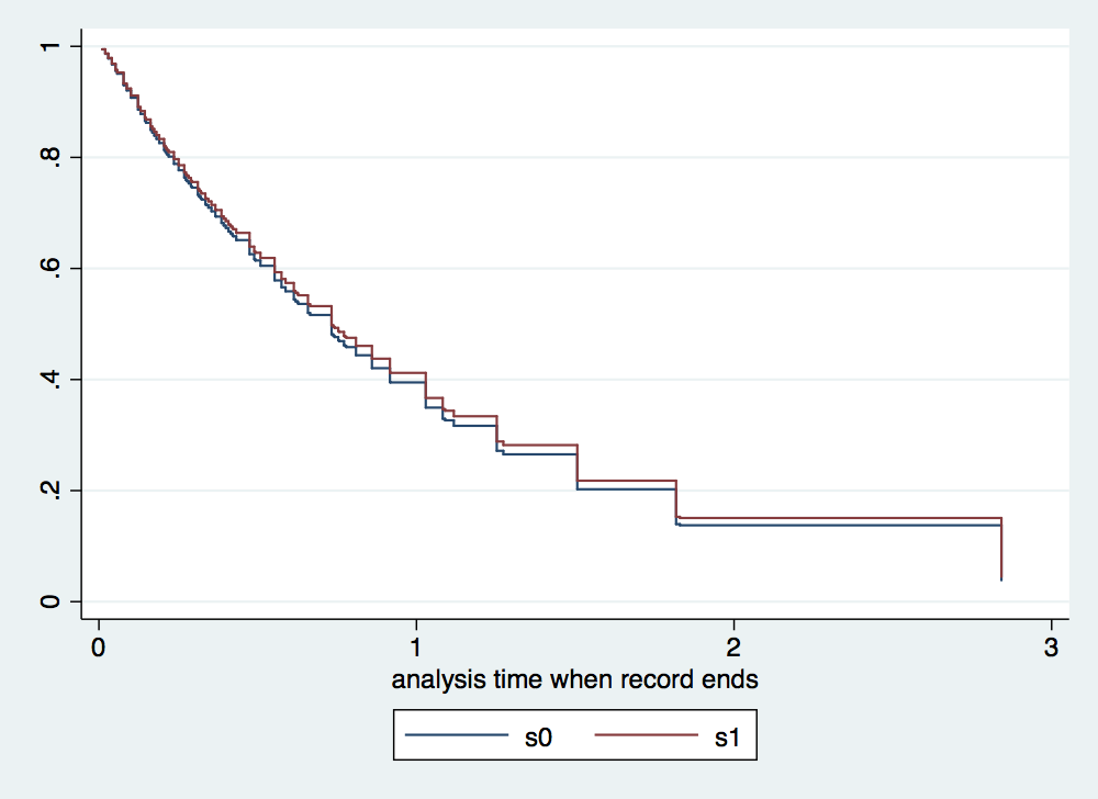
. //ssc install stpm2
. stpm2 gender age, df(3) scale(hazard) eform nolog

Log likelihood = -117.47139                     Number of obs     =        100

------------------------------------------------------------------------------
             |     exp(b)   Std. Err.      z    P>|z|     [95% Conf. Interval]
-------------+----------------------------------------------------------------
xb           |
      gender |   .9540495   .3025159    -0.15   0.882     .5124679    1.776131
         age |   1.000827   .0130148     0.06   0.949     .9756407    1.026663
       _rcs1 |   2.738344   .3655384     7.55   0.000     2.107959    3.557246
       _rcs2 |    1.04388   .1104969     0.41   0.685     .8482989    1.284553
       _rcs3 |    .967567   .0613668    -0.52   0.603     .8544657    1.095639
       _cons |   .3343509    .306433    -1.20   0.232     .0554722    2.015254
------------------------------------------------------------------------------
Note: Estimates are transformed only in the first equation.

. predict s0, meansurv at (gender 0)

. predict s1, meansurv at (gender 1)

. tw line s0 s1 _t, connect (J J) sort //Note different shape as we do not assume