-Life Table
-STNS Stata command
V) Age-Standardised Five-year Net Survival Inference, chohort 1971 VI) Age-Standardised Five-year Net Survival by Deprivation, cohort 1971Note: the data used in the tutorial has been modified from the original source for a teaching purpose and represent breast cancer incident cases between 1971 and 2001 in England
Note: the interpretation of the results is not applicable to the real-world setting
Setting your path and working directory
. clear

. set more off

. cd "/Users/MALF/Desktop"
/Users/MALF/Desktop
Loading the data
. use breast_stns.dta, clear
((All Cases 1971-2001, final datasets))

. set more off

. //browse
Describing the data
. describe

Contains data from breast_stns.dta
  obs:       355,801                          (All Cases 1971-2001, final datasets)
 vars:             7                          3 Mar 2017 14:30
 size:     5,337,015
--------------------------------------------------------------------------------------------------------------------
              storage   display    value
variable name   type    format     label      variable label
--------------------------------------------------------------------------------------------------------------------
sex             byte    %8.0g      sexlb      sex
diagmdy         int     %d                    diagnosis date in days after 1-1-1960 for stns
finmdy          int     %d                    date of last news- either date of death or date of last vital status
agediag         float   %9.0g                 age at diagnosis in years
ageout          float   %9.0g                 age at date of last news in years
dead            byte    %10.0g                vital status at the date of last news
dep             byte    %13.0g     caquintlbl
                                              Deprivation quintile
--------------------------------------------------------------------------------------------------------------------
Sorted by:

. summarize

    Variable |        Obs        Mean    Std. Dev.       Min        Max
-------------+---------------------------------------------------------
         sex |    355,801           2           0          2          2
     diagmdy |    355,801    10552.37    3174.377       4018      15340
      finmdy |    355,801    13138.84    3391.848       4027      16070
     agediag |    355,801    62.30587    14.32948   15.56194   98.99247
      ageout |    355,801    69.38724    13.93029   17.64545   123.9945
-------------+---------------------------------------------------------
        dead |    355,801    .5961788    .4906631          0          1
         dep |    355,801    3.079514    1.391326          1          5
Calendar year at diagnosis
. gen year = year(diagmdy)

. labe var year "calendar year at diagnosis"

. tab year

   calendar |
    year at |
  diagnosis |      Freq.     Percent        Cum.
------------+-----------------------------------
       1971 |      6,061        1.70        1.70
       1972 |      6,436        1.81        3.51
       1973 |      6,293        1.77        5.28
       1974 |      8,527        2.40        7.68
       1975 |      8,689        2.44       10.12
       1976 |      8,667        2.44       12.56
       1977 |      8,844        2.49       15.04
       1978 |      8,881        2.50       17.54
       1979 |      9,408        2.64       20.18
       1980 |      9,463        2.66       22.84
       1981 |      9,746        2.74       25.58
       1982 |      9,954        2.80       28.38
       1983 |      9,936        2.79       31.17
       1984 |     10,183        2.86       34.03
       1985 |     10,707        3.01       37.04
       1986 |     10,801        3.04       40.08
       1987 |     10,647        2.99       43.07
       1988 |     11,141        3.13       46.20
       1989 |     12,112        3.40       49.61
       1990 |     12,721        3.58       53.18
       1991 |     13,821        3.88       57.07
       1992 |     14,241        4.00       61.07
       1993 |     13,816        3.88       64.95
       1994 |     14,032        3.94       68.89
       1995 |     14,260        4.01       72.90
       1996 |     14,952        4.20       77.10
       1997 |     16,020        4.50       81.61
       1998 |     15,857        4.46       86.06
       1999 |     16,589        4.66       90.73
       2000 |     16,553        4.65       95.38
       2001 |     16,443        4.62      100.00
------------+-----------------------------------
      Total |    355,801      100.00
Canlendar year at exit (last known vital status)
Note that in Stata the 1st of January of 1960 = 0
How you will check the consistency of the data?
. gen eyear = year(finmdy)

. labe var eyear "calendar year last follow-up"

. tab eyear dead

  calendar |  vital status at the
 year last |   date of last news
 follow-up |         0          1 |     Total
-----------+----------------------+----------
      1971 |         0        848 |       848
      1972 |         3      1,557 |     1,560
      1973 |         4      2,330 |     2,334
      1974 |         8      2,901 |     2,909
      1975 |        11      3,662 |     3,673
      1976 |        10      4,086 |     4,096
      1977 |         9      4,628 |     4,637
      1978 |        14      4,980 |     4,994
      1979 |         9      5,326 |     5,335
      1980 |        17      5,469 |     5,486
      1981 |        14      5,714 |     5,728
      1982 |        32      5,999 |     6,031
      1983 |        20      6,135 |     6,155
      1984 |        16      6,114 |     6,130
      1985 |        19      6,640 |     6,659
      1986 |        14      6,959 |     6,973
      1987 |        14      7,060 |     7,074
      1988 |        25      7,068 |     7,093
      1989 |        17      7,490 |     7,507
      1990 |        14      7,376 |     7,390
      1991 |        17      7,931 |     7,948
      1992 |        38      8,003 |     8,041
      1993 |        17      8,438 |     8,455
      1994 |        23      8,343 |     8,366
      1995 |        21      8,334 |     8,355
      1996 |        30      8,396 |     8,426
      1997 |        36      8,701 |     8,737
      1998 |        38      8,684 |     8,722
      1999 |        35      8,899 |     8,934
      2000 |        67      9,028 |     9,095
      2001 |        59      9,091 |     9,150
      2002 |        65      8,302 |     8,367
      2003 |   142,964      7,629 |   150,593
-----------+----------------------+----------
     Total |   143,680    212,121 |   355,801


. sum dead finmdy if dead==1 & (finmdy>15705 & finmdy<=16070)

    Variable |        Obs        Mean    Std. Dev.       Min        Max
-------------+---------------------------------------------------------
        dead |      7,629           1           0          1          1
      finmdy |      7,629    15888.17    106.3775      15706      16070
Five age groups are needed for standardisation
. sum agediag, det

                  age at diagnosis in years
-------------------------------------------------------------
      Percentiles      Smallest
 1%     31.72074       15.56194
 5%      39.0308       16.15058
10%     43.49623       16.32307       Obs             355,801
25%     51.34839        16.5065       Sum of Wgt.     355,801

50%     62.27515                      Mean           62.30587
                        Largest       Std. Dev.      14.32948
75%     73.30322       98.96236
90%     81.42094       98.98152       Variance       205.3341
95%     85.48939       98.98973       Skewness      -.0259262
99%     91.62766       98.99247       Kurtosis       2.322189

. egen agegr =cut(agediag), at(0 45(10)75 100) icodes

. recode agegr 0=1 1=2 2=3 3=4 4=5
(agegr: 355801 changes made)

. tabstat agediag, statistics( min max ) by(agegr)

Summary for variables: agediag
     by categories of: agegr

   agegr |       min       max
---------+--------------------
       1 |  15.56194  44.99932
       2 |  45.00205  54.99795
       3 |  55.00068  64.99931
       4 |  65.00205  74.99795
       5 |  75.00069  98.99247
---------+--------------------
   Total |  15.56194  98.99247
------------------------------

. label var agegr "Five age groups for standardisation"
Setting time (note origin and entry)
. stset finmdy, fail(dead==1) origin(time diagmdy) enter(time diagmdy)

     failure event:  dead == 1
obs. time interval:  (origin, finmdy]
 enter on or after:  time diagmdy
 exit on or before:  failure
    t for analysis:  (time-origin)
            origin:  time diagmdy

------------------------------------------------------------------------------
     355801  total observations
          0  exclusions
------------------------------------------------------------------------------
     355801  observations remaining, representing
     212121  failures in single-record/single-failure data
  920269050  total analysis time at risk and under observation
                                                at risk from t =         0
                                     earliest observed entry t =         0
                                          last observed exit t =     12052
Checking the assumptions of time (note _t0)
. list diagmdy finmdy _t0 _t _d _st in 1/10

     +-----------------------------------------------+
     |   diagmdy      finmdy   _t0     _t   _d   _st |
     |-----------------------------------------------|
  1. | 01jan2000   31dec2003     0   1460    1     1 |
  2. | 29jul1998   31dec2003     0   1981    0     1 |
  3. | 30jan1998   31dec2003     0   2161    0     1 |
  4. | 09jul1998   31dec2003     0   2001    0     1 |
  5. | 22dec1998   31dec2003     0   1835    0     1 |
     |-----------------------------------------------|
  6. | 23jan1998   31dec2003     0   2168    0     1 |
  7. | 16jul1998   31dec2003     0   1994    0     1 |
  8. | 07jul1999   31dec2003     0   1638    0     1 |
  9. | 18aug1998   31dec2003     0   1961    0     1 |
 10. | 01sep1999   01oct2003     0   1491    1     1 |
     +-----------------------------------------------+

. scalar  _t = (finmdy - diagmdy) in 1

. display _t
1460
The STRUCTURE OF THE LIFE TABLE (understanding it is really IMPORTANT)
Note: the unit of _age. stns needs _age in days)
. preserve

. clear

. use Lifetable_stns.dta

. list in 1/10

     +----------------------------------------------------------------+
     |   sex   dep       rate   _year    rate_day     _age   yearin~s |
     |----------------------------------------------------------------|
  1. | Males     1   .0124367    1971   .00003405        0       4018 |
  2. | Males     2   .0138573    1971   .00003794        0       4018 |
  3. | Males     3   .0146276    1971   .00004005        0       4018 |
  4. | Males     4    .017085    1971   .00004678        0       4018 |
  5. | Males     5   .0193684    1971   .00005303        0       4018 |
     |----------------------------------------------------------------|
  6. | Males     1    .001033    1971   2.828e-06   365.25       4018 |
  7. | Males     2   .0010931    1971   2.993e-06   365.25       4018 |
  8. | Males     3   .0011213    1971   3.070e-06   365.25       4018 |
  9. | Males     4   .0011925    1971   3.265e-06   365.25       4018 |
 10. | Males     5   .0012982    1971   3.554e-06   365.25       4018 |
     +----------------------------------------------------------------+

. display 11*365.25
4017.75

. restore
In the breast cancer incident dataset we have to generate age at diagnosis in days to merge it with the life table data (rate in days)
. list diagmdy finmdy _t0 _t _d _st agediag in 1/10

     +----------------------------------------------------------+
     |   diagmdy      finmdy   _t0     _t   _d   _st    agediag |
     |----------------------------------------------------------|
  1. | 01jan2000   31dec2003     0   1460    1     1   67.90417 |
  2. | 29jul1998   31dec2003     0   1981    0     1   76.79671 |
  3. | 30jan1998   31dec2003     0   2161    0     1   37.37166 |
  4. | 09jul1998   31dec2003     0   2001    0     1   52.20534 |
  5. | 22dec1998   31dec2003     0   1835    0     1   71.36482 |
     |----------------------------------------------------------|
  6. | 23jan1998   31dec2003     0   2168    0     1   41.65914 |
  7. | 16jul1998   31dec2003     0   1994    0     1   65.86722 |
  8. | 07jul1999   31dec2003     0   1638    0     1    38.8063 |
  9. | 18aug1998   31dec2003     0   1961    0     1   61.37714 |
 10. | 01sep1999   01oct2003     0   1491    1     1   82.03423 |
     +----------------------------------------------------------+

. gen agediagindays = agediag*365.25

. label var agediagindays  "Age at diagnosis in days for Net Survival estimation"

. list diagmdy finmdy _t0 _t _d _st agediag agediagindays in 1/10

     +---------------------------------------------------------------------+
     |   diagmdy      finmdy   _t0     _t   _d   _st    agediag   agedia~s |
     |---------------------------------------------------------------------|
  1. | 01jan2000   31dec2003     0   1460    1     1   67.90417      24802 |
  2. | 29jul1998   31dec2003     0   1981    0     1   76.79671      28050 |
  3. | 30jan1998   31dec2003     0   2161    0     1   37.37166      13650 |
  4. | 09jul1998   31dec2003     0   2001    0     1   52.20534      19068 |
  5. | 22dec1998   31dec2003     0   1835    0     1   71.36482      26066 |
     |---------------------------------------------------------------------|
  6. | 23jan1998   31dec2003     0   2168    0     1   41.65914      15216 |
  7. | 16jul1998   31dec2003     0   1994    0     1   65.86722      24058 |
  8. | 07jul1999   31dec2003     0   1638    0     1    38.8063      14174 |
  9. | 18aug1998   31dec2003     0   1961    0     1   61.37714      22418 |
 10. | 01sep1999   01oct2003     0   1491    1     1   82.03423      29963 |
     +---------------------------------------------------------------------+
Net Survival Estimates at 1, 2, 3, 4, and 5 years after diagnosis
. stns list using lifetable_stns.dta if year(diagmdy)==1971, ///
>         age(agediagindays=_age) period(diagmdy=yearindays) ///
>         strata(dep) rate(rate_day) ///
>         at(1/4 5, scalefactor(365.25) unit(year)) end_followup(3625.5)  ///
>         saving(cohort, replace)
type of estimate: kaplan-meier

         failure _d:  dead == 1
   analysis time _t:  (finmdy-origin)
             origin:  time diagmdy
  enter on or after:  time diagmdy

      Time    Event    Beg.               Net             Net Surv.
    (year)    Time     Total    Fail     Lost             Function     [95% Conf. Int.]
---------------------------------------------------------------------------------------
         1     365     6061     1318        1               0.8013     0.7906    0.8120
         2     730     4742      724        1               0.6949     0.6823    0.7076
         3    1095     4017      575        4               0.6102     0.5966    0.6239
         4    1461     3438      423        2               0.5478     0.5335    0.5621
         5    1826     3013      334        0               0.4992     0.4844    0.5139
---------------------------------------------------------------------------------------
Ploting net surival estimates
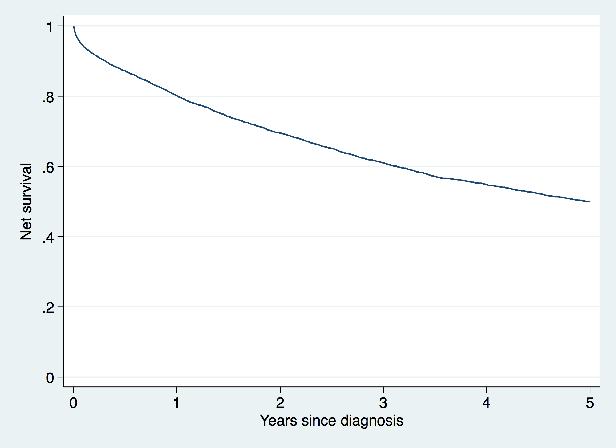
. preserve //Preserve data to plot ten-years net survival

. clear

. use cohort

. drop if time > 1826.25 //Keep just five-year net survival estimates
(767 observations deleted)

. gen year=time/365.25

. twoway (connected survival year, sort msymbol(none)), ///
>         yscale(range(0 1)) ylabel(0(.2)1, labels angle(horizontal) format(%9.1g)) ///
>         ytitle("Net survival") xscale(range(0 5)) xlabel(, val angle(horizontal)) ///
>         xtitle("Years since diagnosis")

. rm cohort.dta

. restore
Net Survival for the cohort of cancer incident cases diagnosed in 1971 and followed-up for 5 years
All what you have to know about STNS: 1. if year(diagmdy) == 1971 2. age and period (specification of the linking variables to merge 1:1 the life table and the incident cases) 3. strata and rate (stratified Net Survial by deprivation) 4. at (years of follow up to compute the Net Survival) 5. scale factor and unit 6. For display end_follow up (in days) and by (agegr dep) 7. saving option (really important!) 8. Please: read carefully the Stata stns help file and the Stata Journal article
. stns list using lifetable_stns.dta if year(diagmdy)==1971, /// > age(agediagindays=_age) period(diagmdy=yearindays) /// > strata(dep) rate(rate_day) /// > at(1 2 3 4 5, scalefactor(365.25) unit(year)) end_followup(5480) by(agegr dep) /// > saving(ASNetcohort_1971, replace) type of estimate: kaplan-meier failure _d: dead == 1 analysis time _t: (finmdy-origin) origin: time diagmdy enter on or after: time diagmdy Time Event Beg. Net Net Surv. (year) Time Total Fail Lost Function [95% Conf. Int.] --------------------------------------------------------------------------------------- agegr=1 Most affluent 1 336 190 18 0 0.9064 0.8649 0.9480 2 719 172 21 0 0.7970 0.7396 0.8544 3 1076 151 14 2 0.7239 0.6600 0.7878 4 1408 135 19 0 0.6230 0.5536 0.6925 5 1801 116 11 0 0.5652 0.4940 0.6363 agegr=1 2 1 347 150 23 0 0.8479 0.7905 0.9053 2 679 127 11 0 0.7756 0.7088 0.8425 3 1084 116 13 0 0.6901 0.6159 0.7643 4 1417 103 8 0 0.6377 0.5605 0.7149 5 1789 95 12 0 0.5584 0.4785 0.6382 agegr=1 3 1 352 138 17 0 0.8783 0.8236 0.9330 2 703 121 15 0 0.7708 0.7004 0.8411 3 1080 106 16 0 0.6559 0.5764 0.7354 4 1446 90 6 0 0.6136 0.5320 0.6953 5 1723 84 6 0 0.5708 0.4877 0.6539 agegr=1 4 1 331 144 13 0 0.9113 0.8645 0.9580 2 640 131 15 0 0.8083 0.7437 0.8729 3 1092 116 13 0 0.7197 0.6459 0.7935 4 1447 103 9 1 0.6582 0.5801 0.7363 5 1620 93 5 0 0.6235 0.5437 0.7034 agegr=1 Most deprived 1 357 126 25 0 0.8034 0.7339 0.8728 2 701 101 14 0 0.6936 0.6130 0.7743 3 1045 87 11 0 0.6074 0.5218 0.6929 4 1430 76 9 0 0.5372 0.4498 0.6247 5 1805 67 6 0 0.4907 0.4028 0.5786 agegr=2 Most affluent 1 365 293 35 0 0.8835 0.8463 0.9207 2 728 258 25 0 0.8008 0.7544 0.8473 3 1093 233 22 0 0.7282 0.6764 0.7801 4 1396 211 17 0 0.6721 0.6172 0.7269 5 1808 194 17 0 0.6165 0.5595 0.6734 agegr=2 2 1 352 231 31 0 0.8690 0.8250 0.9130 2 694 200 17 0 0.7982 0.7456 0.8508 3 1076 183 25 0 0.6925 0.6320 0.7530 4 1458 158 11 0 0.6476 0.5846 0.7105 5 1745 147 14 0 0.5882 0.5233 0.6532 agegr=2 3 1 362 245 33 0 0.8691 0.8263 0.9119 2 728 212 18 0 0.7992 0.7480 0.8503 3 1087 194 22 0 0.7121 0.6541 0.7700 4 1460 172 22 0 0.6244 0.5623 0.6865 5 1797 150 13 0 0.5737 0.5101 0.6373 agegr=2 4 1 353 229 39 0 0.8337 0.7849 0.8825 2 713 190 27 0 0.7190 0.6599 0.7781 3 1031 163 14 0 0.6605 0.5980 0.7231 4 1377 149 12 0 0.6106 0.5460 0.6753 5 1704 137 12 0 0.5604 0.4943 0.6264 agegr=2 Most deprived 1 356 219 32 0 0.8590 0.8120 0.9060 2 716 187 32 0 0.7166 0.6558 0.7775 3 1092 155 23 0 0.6146 0.5487 0.6805 4 1439 132 12 0 0.5626 0.4950 0.6301 5 1820 120 12 0 0.5107 0.4423 0.5790 agegr=3 Most affluent 1 351 308 48 0 0.8518 0.8110 0.8926 2 730 260 37 0 0.7382 0.6874 0.7890 3 1082 223 36 0 0.6256 0.5695 0.6817 4 1444 187 20 0 0.5658 0.5080 0.6236 5 1826 167 16 0 0.5187 0.4598 0.5775 agegr=3 2 1 363 332 47 0 0.8672 0.8294 0.9050 2 730 285 41 1 0.7506 0.7022 0.7990 3 1056 243 33 0 0.6555 0.6021 0.7089 4 1402 210 21 0 0.5972 0.5417 0.6527 5 1826 189 23 0 0.5328 0.4757 0.5899 agegr=3 3 1 343 345 65 0 0.8199 0.7783 0.8615 2 729 280 38 0 0.7174 0.6681 0.7667 3 1084 242 36 0 0.6178 0.5644 0.6713 4 1456 206 29 0 0.5381 0.4828 0.5933 5 1815 177 21 0 0.4807 0.4249 0.5365 agegr=3 4 1 362 338 66 0 0.8145 0.7718 0.8572 2 725 272 58 0 0.6491 0.5965 0.7017 3 1079 214 26 0 0.5779 0.5229 0.6328 4 1451 188 22 0 0.5184 0.4623 0.5745 5 1794 166 13 0 0.4853 0.4286 0.5420 agegr=3 Most deprived 1 333 261 42 0 0.8502 0.8051 0.8952 2 719 219 38 0 0.7142 0.6568 0.7717 3 1089 181 34 0 0.5900 0.5271 0.6528 4 1456 147 23 0 0.5069 0.4425 0.5713 5 1821 124 15 0 0.4542 0.3894 0.5191 agegr=4 Most affluent 1 364 270 39 0 0.8776 0.8346 0.9206 2 686 231 30 0 0.7828 0.7281 0.8375 3 1095 201 28 0 0.6963 0.6339 0.7588 4 1457 173 21 0 0.6325 0.5657 0.6992 5 1806 152 20 0 0.5701 0.5005 0.6397 agegr=4 2 1 361 310 70 0 0.7944 0.7467 0.8421 2 716 240 29 0 0.7181 0.6634 0.7728 3 1074 211 21 0 0.6675 0.6086 0.7264 4 1457 190 25 0 0.6007 0.5380 0.6634 5 1816 165 12 0 0.5786 0.5133 0.6439 agegr=4 3 1 365 329 77 1 0.7872 0.7403 0.8342 2 717 251 39 0 0.6849 0.6303 0.7395 3 1093 212 42 0 0.5678 0.5087 0.6270 4 1383 170 24 0 0.5019 0.4414 0.5625 5 1810 146 17 0 0.4658 0.4034 0.5281 agegr=4 4 1 365 298 67 0 0.7988 0.7500 0.8475 2 719 231 33 0 0.7066 0.6496 0.7636 3 1087 198 36 2 0.5984 0.5360 0.6608 4 1417 160 13 0 0.5700 0.5051 0.6349 5 1791 147 21 0 0.5115 0.4443 0.5786 agegr=4 Most deprived 1 363 213 66 0 0.7141 0.6502 0.7781 2 683 147 30 0 0.5871 0.5159 0.6583 3 1070 117 15 0 0.5351 0.4605 0.6096 4 1420 102 16 1 0.4704 0.3939 0.5470 5 1824 85 14 0 0.4157 0.3378 0.4937 agegr=5 Most affluent 1 361 228 90 0 0.6623 0.5927 0.7318 2 693 138 22 0 0.6058 0.5273 0.6843 3 1092 116 24 0 0.5344 0.4475 0.6212 4 1433 92 14 0 0.5025 0.4092 0.5957 5 1822 78 13 0 0.4602 0.3575 0.5629 agegr=5 2 1 358 240 96 0 0.6522 0.5844 0.7201 2 728 144 42 0 0.5078 0.4329 0.5827 3 1090 102 24 0 0.4249 0.3459 0.5039 4 1461 78 11 0 0.4015 0.3167 0.4863 5 1818 67 11 0 0.3733 0.2842 0.4624 agegr=5 3 1 364 244 102 0 0.6414 0.5733 0.7096 2 704 142 34 0 0.5329 0.4569 0.6090 3 1059 108 23 0 0.4628 0.3816 0.5440 4 1461 85 20 0 0.3992 0.3137 0.4846 5 1826 65 12 0 0.3636 0.2731 0.4541 agegr=5 4 1 349 213 102 0 0.5728 0.4991 0.6464 2 712 111 31 0 0.4586 0.3793 0.5379 3 1081 80 13 0 0.4293 0.3435 0.5151 4 1407 67 22 0 0.3243 0.2401 0.4085 5 1756 45 9 0 0.2873 0.1976 0.3770 agegr=5 Most deprived 1 358 167 75 0 0.6097 0.5261 0.6933 2 725 92 27 0 0.4818 0.3900 0.5737 3 1062 65 11 0 0.4491 0.3506 0.5476 4 1452 54 17 0 0.3390 0.2353 0.4427 5 1796 37 9 0 0.2818 0.1785 0.3850 ---------------------------------------------------------------------------------------
Loading Net Survival estimates and checking consistency
. clear

. use ASNetcohort_1971.dta
((All Cases 1971-2001, final datasets))

. list time if time==5480 & dep==1 & agegr==1 //checking consistency

      +------+
      | time |
      |------|
 123. | 5480 |
      +------+
Undesrtanding the results derived from STNS Stata command
. describe

Contains data from ASNetcohort_1971.dta
  obs:         4,677                          (All Cases 1971-2001, final datasets)
 vars:            20                          28 Mar 2017 15:20
 size:       612,687
--------------------------------------------------------------------------------------------------------------------
              storage   display    value
variable name   type    format     label      variable label
--------------------------------------------------------------------------------------------------------------------
dep             byte    %13.0g     caquintlbl
                                              Deprivation quintile
agegr           float   %9.0g                 Five age groups for standardisation
idgrp           int     %8.0g
time            double  %10.0g                time of events
survival        double  %10.0g                net survival estimate
lower_bound     double  %10.0g                lower_bound of CI of net survival
upper_bound     double  %10.0g                upper_bound of CI of net survival
cum_hazard      double  %10.0g                net cumulative hazard estimate
ch_lower_bound  double  %10.0g                lower_bound of CI of the net cumulative hazard
ch_upper_bound  double  %10.0g                upper_bound of CI of the net cumulative hazard
std_err         double  %10.0g                standard error of net cummulative hazard estimate
n_risk          long    %12.0g                number at risk
n_event         long    %12.0g                number of event
n_censor        long    %12.0g                number censor
dLw             double  %10.0g                increment excess net hazard estimate
dstderr         double  %10.0g                standard error of increment excess net hazard estimate
vnum1           double  %10.0g                weighted observed number of event
vnum2           double  %10.0g                weighted expected number of event
vnumerr         double  %10.0g                term for computation of standard error of excess net hazard estimate
                                                (dstderr)
vden            double  %10.0g                weighted number at risk
--------------------------------------------------------------------------------------------------------------------
Sorted by: agegr  dep  time

. list dep agegr time survival std_err lower_bound upper_bound in 1/10

     +------------------------------------------------------------------------------+
     |           dep   agegr   time    survival     std_err   lower_b~d   upper_b~d |
     |------------------------------------------------------------------------------|
  1. | Most affluent       1     30   .99484885   .00526325   .98458621   1.0051115 |
  2. | Most affluent       1     42   .98962953   .00746324   .97515354   1.0041055 |
  3. | Most affluent       1     71   .98447326   .00916471   .96678966   1.0021569 |
  4. | Most affluent       1     81   .97924578   .01061076   .95888069   .99961086 |
  5. | Most affluent       1    116    .9741107   .01189493   .95140065   .99682076 |
     |------------------------------------------------------------------------------|
  6. | Most affluent       1    151   .96897348   .01306597    .9441592   .99378777 |
  7. | Most affluent       1    184   .96382891   .01415133   .93709605   .99056176 |
  8. | Most affluent       1    216   .95868288   .01516873   .93018107   .98718468 |
  9. | Most affluent       1    218   .95342578   .01613213   .92327998   .98357157 |
 10. | Most affluent       1    232   .94820779   .01705272   .91651611   .97989947 |
     +------------------------------------------------------------------------------+
Keep results for just five-year Net Survival estimates
Q: What do you have to make in order to get 10 years survival?
A: drop if time > ???. Remember: 365.25 x Years (display 365.25*10)
. display 365.25*10
3652.5

. display 365.25*5
1826.25

. drop if time > 1826.25
(1,516 observations deleted)

. bysort dep agegr (time): keep if _n == _N
(3,136 observations deleted)
International Cancer Survival Standard (ICSS) weights (Corazziari I, Quinn M, Capocaccia R. Eur J Cancer. 2004; 40: 2307-16. Standard cancer patient population for age standardising survival ratios.)
Q: Where do you can get the information of the weights for other cancer sites?
A: Check out the Stata do file provide for the exercise and Corazziari et al. European Journal of Cancer. 2004
. gen weight=.
(25 missing values generated)

. *Standard cancer population one (stomach, colon, rectum, liver, lung, breast, ovary, leukaemia)
. replace weight=.07 if agegr==1
(5 real changes made)

. replace weight=.12 if agegr==2
(5 real changes made)

. replace weight=.23 if agegr==3
(5 real changes made)

. replace weight=.29 if agegr==4
(5 real changes made)

. replace weight=.29 if agegr==5
(5 real changes made)
Weighted NET SURVIVAL estimate: from Corazziari et al. European Journal of Cancer. 2004
. bysort /*insert relevant variables*/ dep (agegr): gen s1ASN = (surv*weight)

. list agegr dep surv weight s1ASN

     +-------------------------------------------------------+
     | agegr             dep    survival   weight      s1ASN |
     |-------------------------------------------------------|
  1. |     1   Most affluent   .56518089      .07   .0395627 |
  2. |     2   Most affluent   .61645123      .12   .0739741 |
  3. |     3   Most affluent   .51865789      .23   .1192913 |
  4. |     4   Most affluent   .57010041      .29   .1653291 |
  5. |     5   Most affluent   .46020791      .29   .1334603 |
     |-------------------------------------------------------|
  6. |     1               2   .55835898      .07   .0390851 |
  7. |     2               2   .58824453      .12   .0705893 |
  8. |     3               2   .53280854      .23    .122546 |
  9. |     4               2   .57861378      .29    .167798 |
 10. |     5               2   .37331449      .29   .1082612 |
     |-------------------------------------------------------|
 11. |     1               3   .57082314      .07   .0399576 |
 12. |     2               3   .57370308      .12   .0688444 |
 13. |     3               3   .48073144      .23   .1105682 |
 14. |     4               3   .46575661      .29   .1350694 |
 15. |     5               3   .36356431      .29   .1054337 |
     |-------------------------------------------------------|
 16. |     1               4    .6235172      .07   .0436462 |
 17. |     2               4   .56036181      .12   .0672434 |
 18. |     3               4   .48532551      .23   .1116249 |
 19. |     4               4   .51149627      .29   .1483339 |
 20. |     5               4   .28731031      .29     .08332 |
     |-------------------------------------------------------|
 21. |     1   Most deprived   .49070655      .07   .0343495 |
 22. |     2   Most deprived   .51067644      .12   .0612812 |
 23. |     3   Most deprived   .45424791      .23    .104477 |
 24. |     4   Most deprived   .41574839      .29    .120567 |
 25. |     5   Most deprived   .28176033      .29   .0817105 |
     +-------------------------------------------------------+

. display .70528846*.07
.04937019

. bysort /*insert relevant variables*/ dep (agegr): egen  ASNS = sum(s1ASN)

. list agegr dep surv weight s1ASN ASNS

     +------------------------------------------------------------------+
     | agegr             dep    survival   weight      s1ASN       ASNS |
     |------------------------------------------------------------------|
  1. |     1   Most affluent   .56518089      .07   .0395627   .5316175 |
  2. |     2   Most affluent   .61645123      .12   .0739741   .5316175 |
  3. |     3   Most affluent   .51865789      .23   .1192913   .5316175 |
  4. |     4   Most affluent   .57010041      .29   .1653291   .5316175 |
  5. |     5   Most affluent   .46020791      .29   .1334603   .5316175 |
     |------------------------------------------------------------------|
  6. |     1               2   .55835898      .07   .0390851   .5082796 |
  7. |     2               2   .58824453      .12   .0705893   .5082796 |
  8. |     3               2   .53280854      .23    .122546   .5082796 |
  9. |     4               2   .57861378      .29    .167798   .5082796 |
 10. |     5               2   .37331449      .29   .1082612   .5082796 |
     |------------------------------------------------------------------|
 11. |     1               3   .57082314      .07   .0399576   .4598733 |
 12. |     2               3   .57370308      .12   .0688444   .4598733 |
 13. |     3               3   .48073144      .23   .1105682   .4598733 |
 14. |     4               3   .46575661      .29   .1350694   .4598733 |
 15. |     5               3   .36356431      .29   .1054337   .4598733 |
     |------------------------------------------------------------------|
 16. |     1               4    .6235172      .07   .0436462   .4541684 |
 17. |     2               4   .56036181      .12   .0672434   .4541684 |
 18. |     3               4   .48532551      .23   .1116249   .4541684 |
 19. |     4               4   .51149627      .29   .1483339   .4541684 |
 20. |     5               4   .28731031      .29     .08332   .4541684 |
     |------------------------------------------------------------------|
 21. |     1   Most deprived   .49070655      .07   .0343495   .4023852 |
 22. |     2   Most deprived   .51067644      .12   .0612812   .4023852 |
 23. |     3   Most deprived   .45424791      .23    .104477   .4023852 |
 24. |     4   Most deprived   .41574839      .29    .120567   .4023852 |
 25. |     5   Most deprived   .28176033      .29   .0817105   .4023852 |
     +------------------------------------------------------------------+
Weighted STANDARD ERROR of the net survival estimate. The formula for the the standard error for net survival (se_ns) is derived from the DELTA METHOD based on Clayton and Hills. Statistical Models in Epidemiology, 1993
. gen ns=exp(-cum_hazard) //using the Delta method we ned the cummulative hazard H(t).

. corr ns surv //checking consistency
(obs=25)

             |       ns survival
-------------+------------------
          ns |   1.0000
    survival |   1.0000   1.0000


. gen se_ns=ns*std_err //where std_err is the standard error of the cumulative hazard and ns is the survival estimat
> e from stns

. bysort /*insert relevant variables*/ dep (agegr): gen seASN = sqrt(sum((se_ns*weight)^2))

. //Keep age-standardise estimate by deprivation
. bysort /*insert relevant variables*/ dep (agegr): keep if _n == _N
(20 observations deleted)
95%CIs from Corazziari et al. European Journal of Cancer. 2004 and Clayton and Hills. Statistical Models in Epidemiology, 1993
. gen L95CI=(ASNS/exp(1.96*seASN/ASNS))

. gen U95CI=(ASNS*exp(1.96*seASN/ASNS))
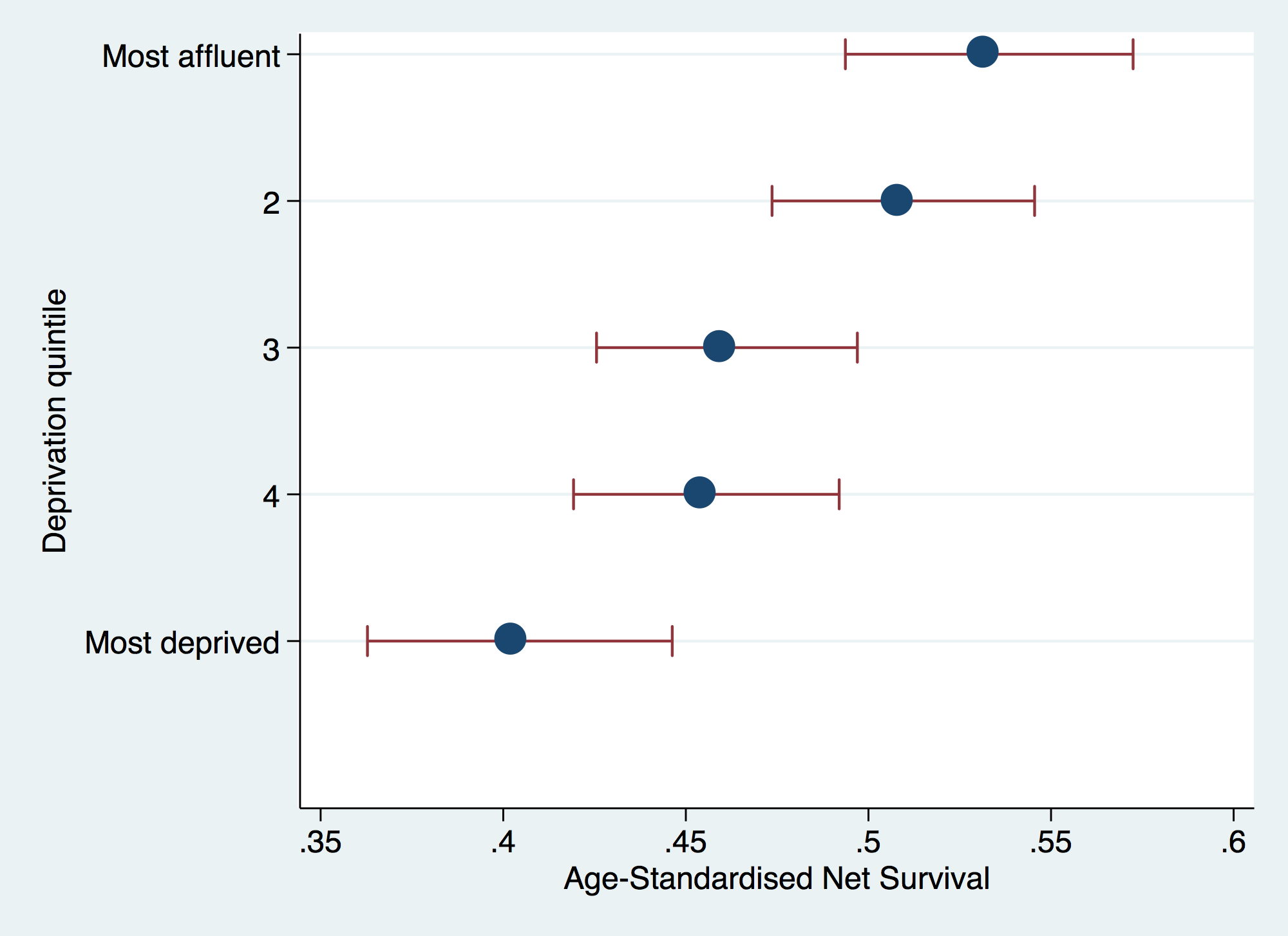
. list dep survival ASNS L95CI U95CI

     +------------------------------------------------------------+
     |           dep    survival       ASNS      L95CI      U95CI |
     |------------------------------------------------------------|
  1. | Most affluent   .46020791   .5316175    .493679   .5724715 |
  2. |             2   .37331449   .5082796   .4736013   .5454971 |
  3. |             3   .36356431   .4598733   .4255474    .496968 |
  4. |             4   .28731031   .4541684   .4192516   .4919932 |
  5. | Most deprived   .28176033   .4023852   .3628127   .4462739 |
     +------------------------------------------------------------+

. eclplot ASNS L95CI U95CI dep, hori estopts(msize(vlarge)) ciopts(msize(vlarge)) yscale(range(1 6)) xline(0,lpatter
> n(dot)) xtitle("Age-Standardised Net Survival")